Lecture 6b

Overview

Prof. Schniter develops first-order Taylor approximations for scalar-, vector-, and matrix-input functions, showing how the gradient determines the local linear model and points in the direction of steepest increase. The lecture connects Taylor remainders and inner products to directional derivatives, extends the formulas to matrices using the Frobenius norm and trace, then works through J(W) = aᵀWb and its NumPy implementation with broadcasting.

Key takeaways

For a vector input, the first-order Taylor model is J(w₀) + ∇J(w₀)ᵀ(w − w₀), with local error of order ‖w − w₀‖₂².
The gradient points in the direction of maximum local increase, and its Euclidean norm equals the maximum slope over all unit-length directions.
For a matrix input, the corresponding linear term is tr(∇J(W₀)ᵀ(W − W₀)), and the squared matrix deviation is measured with the Frobenius norm.
For J(W) = aᵀWb, entrywise differentiation gives ∇J(W) = abᵀ; because the function is linear in W, its first-order Taylor approximation is exact.
NumPy broadcasting computes the outer product abᵀ as a[:, None] * b[None, :], avoiding slow loops over rows and columns.

Chapters

0:00 Gradient Dimensions, RSS Loss, and Efficient Computation

A scalar-valued function of a vector has a gradient vector with one partial derivative per input; a matrix input yields a gradient matrix of the same shape.
For the two-parameter exponential RSS example, the gradient stacks the partial derivatives with respect to A and B.
The example code saves an exponential in a temporary variable so it is computed once rather than repeatedly.

2:30 Scalar Taylor Series and the Local Linear Model

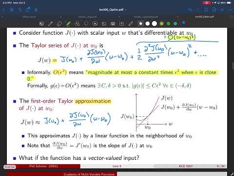
At reference point w₀, the scalar Taylor series begins with J(w₀) plus J′(w₀)(w − w₀), followed by second- and higher-order terms.
The first-order approximation passes through J(w₀) and matches the function’s slope at w₀.
The linear approximation is most reliable near w₀; its error can grow as the distance from the reference point increases.

6:30 Big-O Notation and Dropping Higher-Order Terms

The Taylor remainder is summarized as O((w − w₀)²), indicating that its magnitude is bounded by a constant times the squared deviation near zero.
When the deviation is small, squared and higher powers shrink faster than the first-order term, making them reasonable to omit in a local approximation.
A formal big-O definition uses positive constants and a neighborhood around zero; the lecture emphasizes the informal interpretation for this class.

10:30 Vector Taylor Approximation as a Gradient Inner Product

For a vector input with D components, the first-order expansion sums one partial derivative times its corresponding component’s deviation from the reference vector.
The sum becomes the inner product ∇J(w₀)ᵀ(w − w₀), while the remainder scales with the squared Euclidean norm of the deviation.
Dropping the remainder gives J(w) ≈ J(w₀) + ∇J(w₀)ᵀ(w − w₀), a linear model accurate near w₀.

15:00 Inner Products, Angles, and Local Approximation

For real vectors, the inner product is the product of their norms and the cosine of the angle between them.
A large normalized inner product indicates aligned directions; an inner product near zero indicates near-orthogonality.
Angle-bracket notation generalizes the inner product across vector, matrix, and function spaces, even when the objects cannot be visualized geometrically.

19:00 Directional Derivatives from the First-Order Expansion

To measure the slope at w₀ in a direction u, the lecture considers the change J(w₀ + εu) − J(w₀), divided by a small step ε.
The direction vector u is taken to have unit Euclidean norm, so ε directly represents the distance moved.
Substituting w = w₀ + εu into the Taylor expansion isolates the gradient’s inner product with u.

25:00 Why the Gradient Gives the Steepest-Ascent Direction

As ε approaches zero, the squared-error remainder divided by ε vanishes, leaving the directional derivative ∇J(w₀)ᵀu.
Cauchy–Schwarz bounds the normalized inner product between −1 and 1; its maximum of 1 occurs when u points in the gradient’s direction.
The maximum local slope is ‖∇J(w₀)‖₂, and gradient vectors are perpendicular to the function’s contour lines.

32:00 Matrix Taylor Expansion with the Frobenius Norm and Trace

For a matrix input W with entries Wᵢⱼ, the first-order term sums the entrywise partial derivatives times the corresponding deviations from W₀.
The squared deviations combine into the squared Frobenius norm ‖W − W₀‖F².
The linear term can be written as tr(∇J(W₀)ᵀ(W − W₀)); the trace sums the diagonal entries of the matrix product.

41:00 Turning J(W) = aᵀWb into Scalar Sums

To differentiate without relying on matrix calculus, the bilinear function is written as the scalar sum ΣⱼΣₖ aⱼWⱼₖbₖ.
Differentiating with respect to one entry Wⱼ′ₖ′ leaves only its matching term, giving the partial derivative aⱼ′bₖ′.
Collecting those partial derivatives gives the gradient matrix abᵀ, with each entry formed from one component of a and one component of b.

50:00 The Bilinear Example’s Taylor Approximation Is Exact

Substituting ∇J(W) = abᵀ into the matrix Taylor formula produces the linear change aᵀ(W − W₀)b.
Adding that change to J(W₀) simplifies to aᵀWb, exactly the original function.
The approximation is exact because J(W) = aᵀWb is already linear in W; Taylor approximation adds no higher-order error for this example.

53:00 NumPy Matrix Products and Broadcasting for the Gradient

The function aᵀWb can be evaluated with NumPy matrix products, such as a @ W @ b; the lecture also mentions dot and at-style operations.
The gradient abᵀ can be formed without nested loops using elementwise multiplication with broadcasting: a[:, None] * b[None, :].
Adding a singleton axis turns a into a column-shaped array and b into a row-shaped array, letting NumPy expand them to compatible dimensions.

Summary, takeaways, and chapters were generated by AI from the video's transcript and may contain errors. The video belongs to its creator, Prof. Schniter.