Lecture 2d
 Watch on YouTube →
Overview
Prof. Schniter demonstrates practical linear regression in NumPy and scikit-learn, then shows how training fit, test performance, and categorical feature encoding affect model design. The lecture covers one-hot coding for category-specific intercepts or slopes, explains why using all K indicators with an intercept makes the design matrix singular, and introduces polynomial features as a way to build nonlinear curves with a linear predictor.
Key takeaways
- Use NumPy's least-squares routine or scikit-learn's LinearRegression.fit rather than explicitly calculating (A.T @ A)^-1, which is less efficient and can be numerically fragile.
- Adding features cannot increase least-squares training error because omitting a feature is equivalent to setting its coefficient to zero, but that guarantee says nothing about test-set performance.
- One-hot encoding avoids imposing a false numerical ordering on categories such as Ford, Honda, and BMW; category indicators can control either intercepts or slopes.
- An intercept plus K one-hot indicators is redundant because only K category intercepts are identifiable; omit one indicator to use a baseline category and avoid a singular design matrix.
- Giving each category its own intercept and slope makes separate fitted lines, so observations from one category no longer help estimate another category's model.
- Polynomial regression is linear in its coefficients but can produce nonlinear curves in the raw feature; high-degree models can overfit noisy training outliers.
Chapters
- The general least-squares solution can be expressed using feature covariance, feature-target covariance, and the means of features and targets.
- Simple linear regression uses one feature, so the coefficient matrices and vectors reduce to scalar slope and intercept terms.
- R-squared is 1 for a perfect fit, 0 for a least-squares fit with no explanatory improvement, and can be negative for coefficients worse than least squares.
- Append a column of ones to the feature matrix X using NumPy ones and hstack to create the design matrix A, including an intercept.
- The manual solution computes (A.T @ A)^-1 @ A.T @ y; NumPy uses @ or dot for matrix multiplication, while * performs elementwise multiplication.
- Explicitly forming a matrix inverse is laborious and can be inefficient or numerically fragile for large matrices.
- NumPy's linear algebra least-squares routine returns the coefficient vector without explicitly computing the normal-equation inverse.
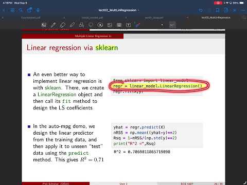
- In scikit-learn, instantiate LinearRegression, call fit(X, y), then use predict(X); the estimator handles the intercept without requiring a ones column in X.
- Training R-squared can be computed as 1 minus mean squared residual divided by target variance; the demonstrated fit is about 0.70.
- An R-squared of 1 requires zero residual sum of squares, meaning every target lies exactly on its prediction.
- Simple linear regression uses one feature, while multiple linear regression uses more than one; the automobile fuel-economy dataset has four features.
- Excluding a feature is equivalent to constraining its coefficient to zero, so least squares with all features can match or improve the training fit.
- Using individual automobile features produces R-squared values around 0.60 to 0.69; the best single feature is about 0.69, compared with about 0.71 for all four.
- The guarantee applies to training error, not to performance on unseen data, where overfitting can make extra features harmful.
- Shuffle the 392 automobile observations, use 300 random samples for training, and reserve the remaining 92 for testing.
- Fit scikit-learn's regression model only on the training set, then separately predict training and test targets.
- The example yields training R-squared around 0.71 and test R-squared around 0.68, illustrating the typical drop on unseen data.
- A test score can occasionally exceed the training score if the test subset is easier, but that is not the usual outcome.
- Categorical values such as Ford, Honda, and BMW should not be encoded as arbitrary numbers like 1, 2, and 3, because that falsely implies an ordering.
- One-hot encoding represents three brands as 100, 010, and 001, creating one binary feature per category.
- When the indicators are used for intercept adjustments, each brand receives a different intercept while sharing a common horsepower slope.
- For iPhone price prediction, Android and iPhone records can be combined with category indicators rather than treated as identical or discarded.
- Multiplying horsepower by each brand indicator gives Ford, Honda, and BMW separate slope coefficients.
- This model keeps one shared intercept while allowing the relationship between horsepower and the target to vary by brand.
- Choosing shared or category-specific intercepts and slopes encodes assumptions about which information can be shared across categories.
- With an intercept and all three brand indicators, the design matrix has redundant parameters: four coefficients represent only three brand intercepts.
- A nonzero coefficient vector such as (-1, 0, 1, 1, 1) can produce zero predictions for every encoded row, demonstrating a null direction and a singular matrix.
- For K categories with an intercept, use K minus 1 indicators; the omitted category becomes the baseline, avoiding the redundancy.
- With Ford and Honda indicators retained, BMW is the baseline intercept, while Ford and Honda intercepts are represented as adjustments to it.
- Giving every brand its own slope and intercept creates effectively separate regression lines for Ford, Honda, and BMW.
- In that setup, Ford observations do not help estimate Honda's or BMW's line, so the procedure partitions rather than pools the data.
- Separate category-specific models may be appropriate when groups differ substantially, but shared parameters can make additional records useful when groups have common structure.
- Starting from one raw feature x, create features such as x, x², and x³, then fit their coefficients with the same linear least-squares method.
- The model remains linear in its learned coefficients, even though its prediction as a function of the raw feature becomes a curve.
- More generally, cosine or other nonlinear transformations can be added as features; neural-network pipelines also create transformed features before a final linear prediction stage.
- Increasing polynomial degree can make a model match training observations closely, including isolated samples that may be measurement errors.
- A ninth-order curve can fit an outlier exactly yet fail to represent the underlying relationship, leading to worse predictions on new data.
- Training fit alone cannot determine the right polynomial order; the next unit will address overfitting and how to assess model complexity.
Transcript excerpt
0:01 Okay, welcome back everyone. Hope you had a good weekend. Um, so let's uh get back to our linear regression notes. Last time we derived an alternate expression for the le squares coefficients. uh we have this expression here for the intercept term and this expression for the slope terms. And here we're using some statistics from our data set like the coariance matrix of the features. The um coariance between the features and the targets and we have the mean of the features and the mean of the target. [clears throat]
0:49 And we also talked about the special case of what's called simple linear regression which is where you use just one feature. And in this case all these these matrices and vectors they turn into scalers. And so we have these simpler expressions. We just have one intercept and one slope coefficient. And we'll be returning to this a little bit later today. We also discussed um the goodness of fit R squared goodness of fit which is a way of understanding from your um your fitted data set whether your fit is good or bad and we have a number R squar where with a perfect fit that would be R square is one. Um if the data was maximally difficult for linear le
1:40 squares and you computed the linear le squares fit anyway you would get r² equals z. Um if you do something foolish and compute coefficients that are worse than least squares then you could get a negative um r 2. So that would be like even worse than um yeah worse than than you would get with le squares. So we talked about that and um so the next thing I talk about is uh just a little bit of discussion of how
This is the start of the transcript. Save this video free for the whole transcript, searchable and time-coded.
Related notes
Summary, takeaways, and chapters were generated by AI from the video's transcript and may contain errors. The video belongs to its creator, Prof. Schniter.