Unit 9a

Overview

The lecture builds character-level autoregressive text generation from first principles using Andrej Karpathy’s Tiny Shakespeare dataset, with 65 character tokens and a time-ordered 90/10 train-test split. It compares empirical bigrams and multinomial logistic regression with n-grams and learned embeddings, showing how embeddings enable longer context efficiently; the lecture ends by motivating attention as a way to use distant, relevant context that recurrent models often struggle to retain.

Key takeaways

Autoregressive language modeling trains on next-token targets formed by shifting a sliding window, then generates text by repeatedly sampling and appending the next token.
Tiny Shakespeare’s 65-character vocabulary makes a basic bigram feasible, but its 27% next-character accuracy and incoherent samples show the limits of conditioning on only one character.
Direct n-gram parameter counts grow exponentially with context length: for 65 character tokens, a three-token context requires about 17 million parameters.
Learned embeddings compress token representations into D dimensions, allowing a T-character context to use T times D input features instead of enumerating every possible context.
On the Shakespeare task, a 10-token embedding-based linear classifier reaches about 32% accuracy and a two-layer MLP reaches about 45%, compared with 27% for the bigram.
Attention addresses a key weakness of recency-based models by letting prediction depend on distant but relevant tokens, such as the subject that determines verb agreement.

Chapters

0:00 Generative Learning and Autoregressive Text Generation

Generative machine learning learns to produce new samples resembling training data, rather than predicting targets from paired features.
Autoregressive text training predicts the next word from preceding words, then shifts a sliding window to form more training examples.
At generation time, the model repeatedly predicts and appends a token, building text from an initial seed.

4:10 Tiny Shakespeare: 65 Character Tokens and Integer Encoding

Andrej Karpathy’s Tiny Shakespeare corpus contains about 40,000 lines and 1.1 million characters, roughly a quarter to a fifth of Shakespeare’s complete works.
The character vocabulary has 65 symbols, including letters, spaces, newlines, and punctuation.
An encoder maps characters to integer tokens and a decoder reverses the mapping; UTF-8 byte encoding was mentioned as an alternative with 256 possible values.

9:12 Time-Based Splits for Shakespeare Text

Unlike ordinary paired datasets, sequential text must not be shuffled because its order carries temporal structure.
The corpus is split chronologically, using the first 90% for training and the final 10% for testing.
A sliding window forms input-context and next-token target pairs, matching the structure of time-series forecasting.

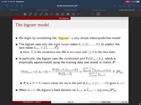
12:19 Training a Character Bigram from Conditional Probabilities

A bigram predicts the next character using only the current token, so each training example is a pair of adjacent characters.
The model estimates conditional probabilities by counting token frequencies and adjacent-token pairs in the training data.
The resulting vocabulary-sized conditional probability table supplies the next-character distribution for a given current token.
Generation samples from that distribution rather than always choosing its most probable character, preserving variation across outputs.

20:51 Comparing Random, Unigram, and Bigram Text Generation

Uniform random generation ignores Shakespeare’s character frequencies, while sampling from the empirical prior captures common letters but not their order.
Next-token prediction accuracy is about 4% for uniform sampling, 15% for the empirical prior, and 27% for the bigram.
Bigram samples begin to show English-like character patterns and word spacing, but still lack coherent words and long-range structure.

25:53 Connecting the Bigram to Multinomial Logistic Regression

The current character is categorical, so multinomial logistic regression represents it with a one-hot vector and predicts the next character with a softmax.
Setting the bias to zero removes a parameter redundancy and yields a probability model parameterized by a weight matrix.
Training minimizes cross-entropy, while empirical bigram probabilities come directly from counts; the learned distributions can be close but generally do not assign exact zero probabilities.

33:58 Why Larger Character N-Grams Become Impractical

An n-gram conditions on T previous tokens, requiring a separate next-token distribution for every possible context.
With 65 possible characters, parameter count grows as 65 to the power of T plus one: about 4,200 parameters for a bigram, 247,000 for a two-token context, and 17 million for three.
This exponential growth makes direct empirical n-grams impractical even for short character histories.

36:30 Learned Embeddings Replace One-Hot Character Representations

One-hot coding assigns each token its own orthogonal direction, even when tokens such as vowels or punctuation share useful similarities.
An embedding maps each of the 65 tokens to a learned real-valued vector in D dimensions, stored as columns in a codebook matrix.
Multiplying the codebook by a token’s one-hot vector selects that token’s embedding; methods such as GloVe can learn embeddings separately, but they are commonly learned jointly with the prediction model.
Stacking T embeddings creates a feature vector of length T times D, making input size grow linearly with context length rather than exponentially.

45:56 PyTorch Embedding Layers and Time-Series Data Loading

PyTorch’s embedding layer maps batches of B by T integer-token sequences to B by T by D floating-point embedding tensors.
The layer avoids explicitly constructing one-hot vectors and repeated embedding matrices, simplifying and speeding up implementation.
A custom time-series dataset can generate sliding-window context and target pairs and support mini-batch training.

49:06 Embedding Model Results and the Need for Long-Range Context

With a context length of 10 and embedding dimension 6, a linear classifier uses about 4,085 parameters, comparable to the roughly 4,300-parameter bigram.
The linear embedding model reaches about 32% accuracy, while a two-layer MLP with 260 hidden units, GELU activations, and batch normalization reaches about 45%, compared with 27% for the bigram.
Generated samples increasingly resemble Shakespeare’s formatting and recognizable words, though they remain far from coherent text.
RNNs, LSTMs, and GRUs add internal memory, but often struggle to preserve information from the distant past.

53:29 Attention Uses Relevant Distant Tokens for Prediction

The 2017 Google paper “Attention Is All You Need” introduced the transformer architecture based on attention.
In “the dog in the park run,” predicting the next character requires linking the verb to the earlier singular subject “dog”; changing it to “dogs” changes the expected verb form.
The nearby phrase “in the park” is less relevant than the distant subject, illustrating why useful context is not always the most recent context.
Attention describes how a target gives weight to the tokens most predictive of it, preparing for the next lecture’s treatment of transformers.

Transcript excerpt

0:01 Okay, we're going to get into a new unit today that is going to start to talk about some more contemporary topics in machine learning. And that's on transformers and large language models. So, >> [clears throat] >> our motivation motivational problem Actually first before I talk about that, our kind of the high level task that we're doing is now going to be different than we've considered so far. So so far we've considered um prediction in the form of either regression or classification. So there we always have data that comes in pairs, we have features and targets and we try to predict the target from

0:49 the features. But now we're going to talk about generative machine learning which is not about prediction at all. It's just about generating random test samples that are similar to those in our training set. And this is an example of an unsupervised task which means you don't have pairs of feature target. You just have features. Um in this case, let's say we have a data set of feature vectors XI and we want to use our model to try to generate a new X that looks a lot like our features XI but yet is not an instance of any of them. Okay, so example would be like I have

1:37 a large data set of cat images and I want to generate a new cat that's not in my data set but you know, it looks like a cat. >> [clears throat] >> Convinces everyone that it's it's actually a cat. Um so that's what generative machine learning is and that's an example of an unsupervised task. We will talk about some other unsupervised tasks in future units. we'll talk about um clustering and we'll talk about um compression, basically some form of

This is the start of the transcript. Save this video free for the whole transcript, searchable and time-coded.

Related notes

Summary, takeaways, and chapters were generated by AI from the video's transcript and may contain errors. The video belongs to its creator, Prof. Schniter.