Lecture 3a
 Watch on YouTube →
Overview
Polynomial model order selection is framed as a trade-off between underfitting and overfitting, illustrated with 70 synthetic samples from a noisy cubic model. The lecture develops shuffled holdout and K-fold cross-validation, explains how NumPy and scikit-learn support the workflow, and uses standard errors and the one-standard-error rule to favor simpler models with performance close to the cross-validation minimum.
Key takeaways
- Training sample MSE cannot reliably select polynomial degree because adding coefficients can only improve the least-squares fit on the training data, even when the model is fitting noise.
- Cross-validation estimates generalization by fitting on one subset and measuring prediction error on samples excluded from that fit.
- Shuffling before K-fold splitting helps prevent pre-existing sample order from making training and test folds systematically different.
- K-fold cross-validation gives every sample a turn as test data while retaining K-1 folds for training, at the cost of fitting each candidate model K times.
- The one-standard-error rule chooses the simplest degree whose average validation error is within one standard error of the minimum, favoring parsimony when measured differences are uncertain.
Chapters
- A degree-D polynomial uses an intercept and coefficients for x through x^D, treating each power as a feature.
- Least squares estimates the coefficients, but the central question is how to choose D from data when the true model is unknown.
- Model order selection balances a simple model against a more flexible one.
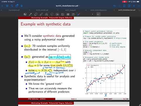
- The example draws 70 input samples uniformly from [-1, 1].
- Targets follow a degree-3 polynomial plus independent Gaussian noise with mean zero and variance 0.16.
- Synthetic data makes the true degree and coefficients known, allowing estimated models to be compared with ground truth.
- Least squares with D=3 produces a curve close to the true cubic, with remaining differences caused by noise.
- A linear model with D=1 cannot reproduce the cubic pattern and underfits.
- A degree-15 fit bends toward individual noisy samples, illustrating overfitting.
- A sufficiently flexible polynomial can pass through every training point, including deviations caused by noise.
- Future samples will contain different noise realizations, so matching training noise can create large prediction errors on new data.
- The desired fit captures the underlying smooth relationship rather than every fluctuation in the training set.
- For each candidate D, least squares fits coefficients and computes training residual sum of squares divided by n, called sample MSE.
- Training MSE falls as D increases because each added coefficient gives the model more flexibility to fit the training data.
- Selecting the degree with minimum training MSE therefore tends to choose the largest degree tested, even when it overfits.
- A simple cross-validation split separates samples into training and test sets.
- Fit coefficients only on the training set, then predict test targets and calculate test sample MSE for each candidate D.
- Choose the degree with the lowest test MSE; unlike training error, test error can rise again as a model begins to overfit.
- Shuffle samples before forming folds so ordered data, such as targets sorted from small to large, do not create mismatched train and test sets.
- Partition the data into K folds, train on K-1 folds, and evaluate on the remaining fold.
- Repeat until each fold has served as the test set once; each run produces a temporary fit used to assess candidate model orders.
- For each candidate degree, average its test MSE across the K folds to obtain a cross-validation performance estimate.
- Five- or ten-fold validation is common, while leave-one-out cross-validation uses K=n and tests one sample per run.
- Repeated K-fold validation reshuffles and repeats the process for a more stable estimate at additional computational cost.
- A nested loop over fold index and model order records test sample MSE for each degree-fold combination.
- NumPy's polynomial fitting and evaluation functions, polyfit and polyval, fit coefficients and generate predictions.
- scikit-learn's KFold utility generates train and test indices, with shuffling enabled; averaging across folds yields one score per degree.
- The standard error of an average is the sample standard deviation of the measurements divided by the square root of the number of measurements.
- For K-fold estimates, the sample standard deviation uses the K fold errors and an unbiased variance denominator of K-1.
- Error bars show each degree's mean test MSE plus or minus one standard error, indicating how variable the fold-based estimate is.
- First identify D_min, the degree with the lowest average cross-validation MSE.
- Set a threshold at D_min's average MSE plus its standard error, then choose the smallest degree whose average error is at or below that threshold.
- This rule can avoid selecting a needlessly complex degree when several models have statistically similar validation performance.
- Exam papers are handed out after class, with remaining papers available the following week.
- A student asks whether a homework Python file must be uploaded to GitHub; the answer is no, it can be printed and does not need to be run.
- For difficulty with an exam concept, Prof. Schniter suggests discussing it with a TA or attending Wednesday office hours from 1 to 3.
Transcript excerpt
0:02 Welcome back everyone. I have the exams. I'm going to pass them out um just at the end of lecture and if you have to leave that's fine. I'll bring them next week as well. Um so we're going to start today with uh the first real machine learning lecture. I think until now we've just been doing very basic like numerical analysis that you might have seen in other classes, signal processing classes, things like that. [clears throat] So um the motivation uh for [clears throat] or at least how we're going to present this material is motivated by our polomial model that we talked about last time. So we said that in the case that
0:51 you had um a single feature. You can of course do this with multiple features too, but just for simplicity we'll talk about a single single feature. Um, you could make a model that has the intercept coefficient plus beta 1 times the raw feature x plus beta 2 * x^2 and then you could keep adding more coefficients with higher and higher powers of x. So in some sense, you know, all we're given is x and we are sort of synthetically making these new additional features by taking that x and raising it to higher powers. Um [clears throat]
1:38 and so in this case the model parameters for us are going to be all these different betas. We have a total of d + one. Um d is the degree of this polomial here. [snorts] And um and we know [clears throat] exactly how to find these betas because last time we said that we can just think of each of these as a feature. So this could be like the feature index by j= 1, j= 2 all the way to j equals d. In other
This is the start of the transcript. Save this video free for the whole transcript, searchable and time-coded.
Related notes
Summary, takeaways, and chapters were generated by AI from the video's transcript and may contain errors. The video belongs to its creator, Prof. Schniter.