Lecture 3c
 Watch on YouTube →
Overview
The lecture derives the conditional mean-squared-error decomposition into irreducible noise, squared bias, and prediction variance, using linearity, independence, and conditional expectation. Polynomial least-squares examples with degrees 1, 3, and 14 show how model complexity trades bias for variance, while a linear-regression result quantifies average variance as (D+1)σ²/N when training data are plentiful.
Key takeaways
- At a fixed test feature x, conditional MSE equals σ² + bias(x)² + variance(x), assuming zero-mean noise independent of features and training data.
- The irreducible error σ² remains even when the predictor exactly matches the true function, because independent test noise cannot be predicted.
- Increasing model complexity can reduce approximation bias, but the degree-14 polynomial example shows that it can greatly increase prediction variance when training data are limited.
- In the polynomial demonstration, 100,000 repeated least-squares fits make the degree-3 and degree-14 average predictions match the true cubic, even though individual degree-14 fits vary widely.
- For least-squares linear regression with sufficient data, average variance scales as (D+1)σ²/N, so adding parameters raises variance and adding training samples lowers it.
- Underfitting occurs when the prediction model has fewer features than the true model; extra irrelevant features need not create bias under the stated assumptions, though they can increase variance.
Chapters
- Reviews linearity of expectation, factorization for independent variables, variance as E[Z²] minus E[Z]², and conditional expectation.
- Defines the target as y = f(x) + ε, with zero-mean noise of variance σ² independent of the features.
- Treats training data and test data as independent, making fitted coefficients β̂ random because they depend on random training samples.
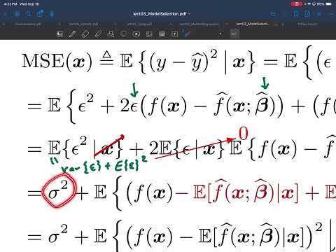
- Starts from MSE conditioned on a fixed test feature x and substitutes y = f(x) + ε.
- Expands the squared prediction error into an ε² term, a cross term involving ε and f(x) − f̂(x), and a squared model discrepancy.
- Uses linearity to split the conditional expectation across the three terms while holding x fixed.
- Identifies test noise ε and fitted coefficients β̂ as the remaining random quantities after conditioning on test feature x.
- Training-test independence makes ε independent of β̂ and functions of β̂, so the cross-term expectation factors into separate expectations.
- Zero-mean noise gives E[ε|x] = 0, eliminating the cross term; E[ε²|x] = σ² supplies the irreducible-noise contribution.
- Adds and subtracts the conditional mean prediction E[f̂(x)|x] inside the squared model discrepancy.
- Expands the centered expression into squared bias, prediction variance, and a cross term.
- The cross term vanishes because the centered prediction has conditional expectation zero, leaving the two components to add.
- Defines bias at fixed x as the difference between the average prediction and f(x); zero-mean noise makes f(x) the average target.
- Defines prediction variance as E[(f̂(x) − E[f̂(x)|x])²|x], measuring variation across possible fitted models.
- Summarizes conditional MSE as σ² plus squared bias plus variance, then averages over the distribution of test features to obtain a scalar performance measure.
- Compares a linear predictor with a cubic true function, using least squares to fit β₀ and β₁ from each training set.
- Averages predictions across 100,000 simulated training experiments to estimate the expected fitted curve.
- The average line differs from the true cubic at most x values, illustrating underfitting bias; prediction variability also grows toward the feature-range extremes.
- Fits a degree-3 polynomial with β₀, β₁, β₂, and β₃ across repeated training samples.
- The average fitted curve matches the cubic truth, so the bias is zero, although individual fits still vary because of noisy training data.
- Compared with degree 1, the error bars are larger, demonstrating the variance cost of increasing model complexity.
- Repeats the simulation with a degree-14 polynomial and averages predictions over 100,000 fits.
- The average curve still matches the true cubic, but individual fits deviate substantially, especially near the edges of the feature range.
- The example shows that adding parameters beyond the true model order can preserve zero bias while sharply increasing variance.
- A tightly grouped set of darts away from the bullseye represents low variance with systematic bias.
- Darts centered on the bullseye on average but widely spread represent zero bias with high variance.
- Bias describes average directional error, while variance describes spread around the average prediction.
- For least-squares regression with D features, fewer than D+1 training samples can yield non-unique coefficient solutions with differing test performance.
- With enough samples, using fewer features than the true model causes nonzero bias; using at least the true feature set can remain unbiased, even with extra irrelevant features.
- When N is large relative to D, average prediction variance is (D+1)σ²/N: more parameters increase variance, while more training samples reduce it.
- The closing trade-off curve places the preferred model complexity between underfitting, where squared bias is high, and overfitting, where variance is high.
Transcript excerpt
0:00 looking behind. >> Okay, welcome back everyone. Um, [clears throat] so today is going to be an important day where we'll learn about um the bias variance trade-off which is one of the most uh important concepts for this entire semester. Uh so last time we reviewed a bit about probability and random variables and expectation and we're going to be using this today. So let me just um kind of summarize what we did with expectation. So we we defined what it is but then we said it's mostly enough for us to focus on a couple key properties. The first is linearity [clears throat] which basically says the expectation operator is linear. So the expectation of
0:47 um a linear combination or you could say the expectation of a sum is the same as a sum of expectations. And the other thing we learned is that if you have an expectation of a product of two things where those two things are independent statistically independent of each other, you can break that into the product of their individual expectations. [clears throat] Uh we also learned about the the sample variance. Um we'll be using this equation later today as well. So the variance of a random variable is the expected squared value minus the squared expected value. [clears throat] Um and then we learned about or we
1:35 reviewed [clears throat] conditional expectation where you're doing that statistical average but given that some other event is um in effect or you could say uh given some other random variable being held fixed. [clears throat] Um and the main thing is that when you're doing highlight this so when you're doing this expectation and you're holding you're conditioning on a you're holding a fixed then terms like this f of a can be treated as
This is the start of the transcript. Save this video free for the whole transcript, searchable and time-coded.
Related notes
Summary, takeaways, and chapters were generated by AI from the video's transcript and may contain errors. The video belongs to its creator, Prof. Schniter.