EDF9850_Example3_Part4
 Watch on YouTube →
Overview
Lesa Hoffman compares cluster-mean-centering with constant-centering in multilevel models, showing how the choices change intercept and level-two interpretations while preserving fitted results when models contain only fixed effects. She demonstrates predicted-value plots for continuous SCES and binary non-white status, then connects the methods to project planning, missing-data decisions, and presentation requirements.
Key takeaways
- With no random slopes, cluster-mean and constant-centered versions of the model can produce identical likelihoods, effect sizes, and predictions even though their level-two coefficients have different interpretations.
- Cluster-mean centering a binary predictor creates a level-one zero at the school's proportion, which is not a possible individual value; plotting the original zero-versus-one variable can make results clearer.
- A contextual effect compares outcomes across school contexts while holding a student's original predictor value fixed; it cannot be directly read from a plot whose x-axis is centered separately within each school.
- Parallel predicted lines encode the fixed-slope assumption; random slopes are needed to investigate whether individual-level effects, such as the non-white achievement gap, vary by school.
- In the class's standard multilevel models, cases missing any analysis variable are excluded, and a missing school-level predictor can remove information for an entire cluster.
- Hoffman's project workflow prioritizes data and variable selection first, a project plan due the next week, revisions two weeks later, and commented-output review by the end of October.
Chapters
- Lesa Hoffman opens with a brief account of her son's childhood term “Dr. Mama,” then returns to centering and multilevel modeling.
- The lecture resumes at model 4C, which uses cluster-mean-centered level-one predictors instead of the constant-centered versions discussed earlier.
- Model 4C centers student SCES around the school mean and non-white status around each school's proportion of non-white students, with both school means included at level two.
- Because the model has no random slopes, it assumes the SCES and non-white effects are identical across schools; Hoffman identifies random effects as a later topic.
- Changing centering changes the intercept's reference point. For binary non-white status, cluster-mean centering makes zero a school's proportion, which is not a possible individual response.
- The two fixed-effect parameterizations are likelihood-equivalent: they have the same minus-two log likelihood, effect sizes, and predictions, while their level-two coefficients represent different quantities.
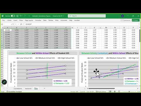
- Hoffman uses an Excel sheet in the Unit 3 download to combine model coefficients and hypothetical predictor values into predicted outcomes.
- For continuous SCES, she selects low, average, and high values using plus or minus one standard deviation: about 66 for within-school SCES and 0.41 for school-mean SCES.
- She holds non-white status at zero to plot SCES effects for white students, and explains that adding a binary predictor's effect would shift the plot without changing its slopes.
- The example draws on High School and Beyond data and an article about approaches to clustered data; Claude-generated R code and the original Excel sheet are also provided.
- With cluster-mean-centered SCES on the x-axis, separate lines for low-, medium-, and high-SCES schools show the within-school slope and the between-school differences.
- That within-centered plot cannot directly show a contextual effect because zero refers to each school's different mean, not to the same student SCES across schools.
- Using original SCES on the x-axis makes equal student values comparable across schools and permits a contextual-effect comparison at a fixed student SCES.
- The example distinguishes a between-school slope of 5.33 from the contextual effect; plotted line spacing depends on the selected scale and need not equal a coefficient numerically.
- For the binary non-white predictor, Hoffman uses school proportions of 0.05, 0.30, and 0.55 to represent low-, medium-, and high-proportion schools.
- A cluster-mean-centered plot requires hypothetical individual values such as 0.30, even though a person cannot have that binary value; the original zero-versus-one plot is easier to interpret.
- The model estimates a negative individual-level association for non-white status but a positive contextual association with attending a school with a higher proportion of non-white students.
- Parallel lines follow from the no-interaction, fixed-slope assumption; random slopes can test whether the non-white achievement gap varies across schools.
- Hoffman recommends asking advisors and program colleagues for longitudinal or clustered data that could support a conference presentation or manuscript.
- When suitable local data are unavailable, students can collaborate across research areas or use public-use datasets; she identifies High School and Beyond as one available source.
- Whether a project requires IRB review depends on how data were collected and whether they are deidentified; new data collection requires approval, while previously collected data may qualify for exemption.
- Hoffman says students should not add her to IRBs or share raw datasets with her; she may only need to review analysis output.
- The project plan is due the following week, with revisions scheduled two weeks later; students should identify their data and variables even if the plan is not yet final.
- For the models covered in class, rows missing any analysis variable are excluded, so Hoffman advises checking missingness during descriptive analysis before fitting models.
- Missing level-two characteristics are especially consequential because one missing cluster value can affect every case in that school.
- Multilevel SEM can handle predictor missingness by modeling predictors as outcomes, but Hoffman describes it as a substantially different modeling and software workflow.
- A scattered “Swiss cheese” pattern of missing values can leave too few complete cases, making a simple deletion strategy unsuitable for a publishable analysis.
- Hoffman offers to discuss severe missingness and points to Mplus for multilevel SEM; lavaan in R lacks random-slope support for more complex models, while brms offers a Bayesian alternative.
- By the end of October, students should send commented output for a project check-in so Hoffman can catch modeling problems before presentations.
- The instructor plans to share an anonymized document of students' within-, between-, and contextual-effect examples, and expects to post Lecture 4 slides and a shorter video soon.
- The final project is a presentation rather than a required paper; written components are the project plan, check-in materials, and one peer review.
- Hoffman favors presentations because students can explain their models and findings without polishing a manuscript before analyses are settled; students can develop the work into a paper later.
- Students may submit a revised presentation recording for additional points if the initial presentation does not go as planned.
- The class ends with a reminder to work on project plans before the next session, which Hoffman expects to hold in person.
Transcript excerpt
0:00 There we go. It's now recording. We're back. Okay. Excellent. So, you all got your chips or broccoli or whatever you're you're needing to get through the rest of this. We're not going the whole time. I'll just tell you that right now. I can't feed my kid dinner at 8:00 and expect him to get to bed by 8:45. It's not happening. So, we we'll be ending on the early side. I have to be uh Dr. Mommy. There's a story behind that, by the way. That's sort of how I refer to myself when I'm in a dual role. But my when my son was two, he went through this phase where he would call me Dr. Mama. Like he found out that I was a doctor and he just called me that for like a month. And then he tried to tell him that, "No, your daddy's a doctor, too." And he just would not believe us. Like no, that's not no doctor. Dad, no. No. And like then it occurred to me. We took him to
0:49 the pediatrician and that office was staffed fully by women. So in his world view, only mommies could be doctors, which I just loved and I encouraged. So I was like, "Yeah, yes, Hugh, but we'll make an exception for you if you want to be a doctor someday." But you know, yes, only mommies. So Dr. Mama, Dr. Daddy, absolutely not. Then of course he took um he served as a a test subject for someone who was learning how to administer the PPVT vocabulary test to children. And they had an item which was pick out the doctor and none of the women doctors were in the picture. It was like dudes with stethoscopes or like in women with like dresses doing other
This is the start of the transcript. Save this video free for the whole transcript, searchable and time-coded.
Related notes
Summary, takeaways, and chapters were generated by AI from the video's transcript and may contain errors. The video belongs to its creator, Lesa Hoffman.