Control Systems -- Lecture 20: Design using Frequency Response Techniques
Overview
Christian Hubicki shows how Bode plots can guide practical control design by predicting a system’s sinusoidal output magnitude and phase, then adjusting a controller to improve tracking. Using a linearized pendulum in MATLAB, he compares a PD controller with lead compensation, connecting Bode behavior to time-domain simulations, resonance, and pole-zero placement.
Key takeaways
- For a sinusoidal input to an LTI system, the Bode magnitude predicts the steady-state output amplitude ratio and the Bode phase predicts its timing offset.
- A linearized pendulum with mass and length equal to 1 has natural frequency √(9.81) ≈ 3.13 rad/s; without damping, driving near that frequency creates a large resonance peak.
- For H(s) = K(s + z), the derivative gain is Kd = K and the proportional gain is Kp = Kz, allowing damping and response strength to be tuned through different parameters.
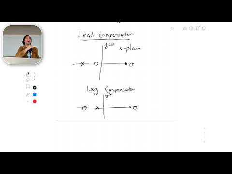
- A lead compensator places its zero closer to the origin than its pole, raising phase over a frequency band; reversing their order creates a lag compensator.
- MATLAB’s feedback command builds the unity-feedback closed-loop transfer function, lsim tests arbitrary inputs such as sin(t), and bode checks predicted magnitude and phase.
Chapters
- Christian Hubicki lists steady-state error, root locus, and Bode plots as exam topics, with an exam review planned for the next class.
- The lecture shifts from constructing Bode plots to using them to improve a controlled system’s response to sinusoidal inputs.
- A sinusoidal input passes through a controller H(s) and plant G(s) in a unity-feedback loop.
- For an LTI system, the output keeps the input frequency but may have a different magnitude and phase.
- Examples such as precisely following a back-and-forth path motivate why tracking performance matters.
- The pendulum receives control torque τ, with angular acceleration modeled using gravity and torque divided by mL².
- Applying the small-angle approximation sin(θ) ≈ θ gives G(s) = Θ(s)/Τ(s) = 1/[mL²(s² + g/L)].
- The model is a linearized plant suitable for transfer-function and frequency-response analysis.
- Hubicki chooses a PD controller H(s) = K(s + z), which contributes a gain and a zero at s = −z.
- MATLAB’s ZPK representation specifies transfer functions through zeros, poles, and gain.
- For the example plant, the undamped poles are at ±j√(g/L).
- The MATLAB example sets pendulum mass and length to 1 and uses Earth gravity.
- The plant is entered with ZPK using no zeros, imaginary poles, and gain 1/(mL²).
- The initial controller uses K = 1 and z = 10, placing its zero at −10.
- The closed-loop transfer function is G(s)H(s)/[1 + G(s)H(s)] for unity feedback.
- MATLAB’s feedback command forms the closed-loop system with forward path G·H and feedback value 1.
- A step response demonstrates that the PD controller’s derivative action damps the pendulum’s oscillation.
- MATLAB’s lsim command simulates the closed-loop response to a sampled input, here sin(t).
- At an input frequency of 1 rad/s, the output amplitude is about half the input amplitude.
- An amplitude ratio of 0.5 corresponds to 20log₁₀(0.5), approximately −6 dB, matching the Bode magnitude near that frequency.
- The Bode plot shows a resonance peak because the pendulum model has imaginary poles and no inherent damping.
- For mass and length equal to 1, the natural frequency is √(g/L) ≈ √9.81 ≈ 3.13 rad/s.
- Driving the undamped plant near 3.13 rad/s produces a very large response, while the PD controller’s derivative action reduces the peak.
- At 1 rad/s, the closed-loop Bode plot shows roughly −5 dB gain and about 2 degrees of phase lead, consistent with the time response.
- At 10 rad/s, the magnitude is around −20 dB, corresponding to an output amplitude about one tenth of the input.
- The phase plot predicts substantial lag at higher frequency, helping explain why sinusoidal tracking deteriorates.
- Expanding H(s) = K(s + z) gives Kd = K and Kp = Kz, so the derivative and proportional gains can be adjusted separately through K and z.
- Increasing derivative gain adds damping; proportional gain mainly increases the response strength and speed.
- A trial setting of K = 50 and z = 4 gives Kd = 50 and Kp = 200, producing a step response with only slight overshoot.
- To reduce phase lag near a target frequency, the lecture proposes adding a zero first and a pole at a higher break frequency.
- The example lead network is G₂(s) = (s/20 + 1)/(s/100 + 1), with a zero at −20 and a pole at −100.
- The zero’s lower break frequency makes the phase rise before the pole causes it to fall; the Bode plot confirms the intended shape.
- Applying G₂ before the closed-loop system gives the response G₂·GCL, and the Bode plot shows phase near zero around 30 rad/s.
- The compensated magnitude is about 4 dB higher at that frequency, an amplitude ratio of 10^(4/20), or roughly 1.6.
- Placing G₂ inside the feedback controller also improves phase behavior; the example reduces the phase offset from about 45 degrees to about 13 degrees.
- A lead compensator adds phase lead, with its zero closer to the origin than its pole; the example places them at −20 and −100.
- Reversing the ordering creates a lag compensator, which adds phase lag.
- Compensators can reshape gain and phase at selected frequencies, while a linear system’s output magnitude can also be scaled by scaling its input.
Transcript excerpt
0:00 All right, I think we're almost ready. >> Okay, I think we got it. All right. Um, so I was hoping to pass back. I have I have all the exams passed back today. My TA, he has to be out of town for a work commitment, so he can't be back to pass the quizzes, but I'm sure he's working hard on those. Okay. So, for today, I'll pass back the quizzes at the end of Gosh, I don't have much time. Uh, thankfully, there aren't that many of you here today. I guess I'm not Okay, I need to make this class more exciting then. Okay. All right. All right. We'll make it more exciting. Okay. I know that we have our exam coming up. We're going to have our exam review next class. So today is the 20 20
0:54 6 112. We have our exam review next class. We've got all of our exams to pass back today. Okay. And just as a reminder, the exam is going to cover, steady state error, root locus. Okay. The ability to understand it when you look at one, be able to sketch one rough and detailed. And we talked about
1:44 what that means. And finally, some frequency response techniques, which means bodie plots. Okay, so that's the that's material I want to cover for the exam. We've mentioned this before. Exactly the same materials covered on the quiz. Exactly the same material that's being covered on the homework. I will get you out as quickly as I can the practice exams soon. As you probably noticed that the practice exams are probably very helpful for doing what's on the real exam. Okay, I see some nodding. So, okay, try to give you all the tool tools that you
2:31 need
This is the start of the transcript. Save this video free for the whole transcript, searchable and time-coded.
In this course
Related notes
Summary, takeaways, and chapters were generated by AI from the video's transcript and may contain errors. The video belongs to its creator, Christian Hubicki.