CMU Introduction To Deep Learning 11-785, Fall 2026: Lecture 24
Overview
The lecture develops Generative Adversarial Networks (GANs) from their motivation: maximum-likelihood training of a VAE-style generator does not directly test whether novel samples look like the training data. It explains the generator-discriminator minimax game, derives the optimal discriminator and the connection between the original GAN objective and Jensen-Shannon divergence, then motivates Wasserstein GANs with a 1-Lipschitz critic to provide useful gradients when distributions have disjoint support.
Key takeaways
- The original GAN discriminator’s optimal output is p_data(x) / (p_data(x) + p_g(x)); when the distributions match, it outputs 0.5 everywhere.
- GAN training compares real and generated distributions through an adversarial game, rather than requiring each generated sample to reproduce a particular training example.
- KL and JS divergences can provide poor generator feedback when real and generated distributions have disjoint support: KL may be infinite and JS may stay constant as the distributions move closer.
- Wasserstein distance measures the minimum cost of transporting probability mass and can vary smoothly with the separation between distributions.
- WGAN replaces the probability discriminator with a 1-Lipschitz critic that maximizes the difference between average real and generated scores; a gradient penalty on interpolated samples can enforce the constraint.
- Mode collapse occurs when a generator repeatedly produces a narrow set of outputs, potentially just one face; encouraging diversity or conditioning on class labels can help address it.
Chapters
- The opening minutes contain informal campus conversation before the lecture begins.
- At about 6:26, the class starts with a small in-person attendance and a check for Zoom participants.
- The lecture reviews diffusion models and the distinction between generative and discriminative models.
- Explicit models compute sample probabilities, while implicit models provide a way to draw samples.
- GANs and diffusion models are introduced as implicit generative approaches.
- A VAE maps samples from a Gaussian latent distribution through a decoder to produce data.
- The decoder transforms a simple latent space into a curved, fuzzy data manifold.
- The encoder helps infer latent variables for training examples, while the decoder is the generative component.
- Maximum-likelihood training raises the probability of observed training examples but does not directly evaluate arbitrary generated samples.
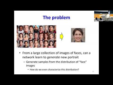
- A generator can assign high probability to training faces yet behave unpredictably for latent inputs not associated with those examples.
- High-dimensional image spaces remain sparsely covered even with very large datasets, so collecting more examples does not test every possible output.
- A GAN pairs a generator that transforms random latent samples with an adversary, the discriminator, that judges real versus generated data.
- The generator is compared with real data at the distribution level rather than by matching each training example to a particular latent code.
- A discriminator that cannot distinguish generated samples from real faces provides evidence that the generator has learned face-like outputs.
- Real training examples are labeled real, while samples produced by the generator are labeled fake.
- The discriminator maximizes log D(x) for real examples and log(1 - D(x)) for generated examples.
- The generator receives feedback through the discriminator rather than maximizing the likelihood of individual training images.
- The original GAN objective combines the expected log discriminator score on real data with the expected log(1 - D) score on generated data.
- The discriminator maximizes this objective, while the generator minimizes it to make generated samples score as real.
- Training alternates between updating the discriminator and updating the generator while holding the other component fixed.
- For real-data density p_data(x) and generator density p_g(x), the optimal discriminator is p_data(x) / (p_data(x) + p_g(x)).
- Where real and generated densities overlap equally, the discriminator outputs 0.5; where real data dominates, its output approaches 1.
- The discriminator’s decision boundary follows the relative densities of the two distributions.
- After the discriminator learns to separate the current distributions, the generator shifts its output toward regions classified as real.
- The discriminator must then adapt to the shifted generator distribution, creating an iterative contest rather than a one-time classification step.
- At the ideal equilibrium, the generated distribution matches the real distribution and the discriminator cannot do better than output 0.5.
- Substituting the optimal discriminator into the GAN objective produces a quantity related to the Jensen-Shannon (JS) divergence between real and generated distributions.
- Unlike KL divergence, JS divergence is symmetric and remains finite when one distribution assigns zero probability where the other does not.
- The original GAN therefore minimizes a divergence between distributions when the discriminator is optimized.
- When p_g equals p_data, the optimal discriminator is 0.5 everywhere and provides no further generator gradient.
- A discriminator that is random or overly certain can also provide unhelpful gradients, so a flat discriminator score does not always indicate successful convergence.
- The minimax game can oscillate or become unstable if either network updates too aggressively or fails to track the other.
- The lecture contrasts VAE training, described through KL-based likelihood objectives, with GAN training through a discriminator and the JS divergence.
- VAEs are presented as comparatively easy to train but prone to blurry outputs; GANs can produce sharper results but are harder to stabilize.
- Examples from GAN research between 2014 and 2019 illustrate substantial gains in generated image quality.
- A saturated sigmoid discriminator can output values near 0 or 1 with almost zero slope, leaving the generator little useful feedback.
- A random discriminator is also unhelpful because its scores do not indicate which output changes would make a sample more realistic.
- The discriminator must distinguish effectively while retaining gradients that guide the generator toward real-data regions.
- For real data concentrated at 0 and generated data concentrated at θ, KL divergence can be infinite whenever the distributions do not overlap.
- JS divergence stays finite but can remain constant as separated distributions move closer, so it may not provide a useful gradient for the generator.
- The lecture’s example shows why a divergence value alone may fail to reflect whether one generated distribution is nearer to real data than another.
- The Wasserstein, or Earth Mover, distance treats distributions as piles of probability mass that must be transported into one another.
- Its cost depends on both how much mass moves and how far it travels, distinguishing distributions that KL or JS may treat similarly.
- In the point-mass example, the distance changes smoothly as the generated point approaches the real point, giving a more informative training signal.
- A transport plan π(x,y) specifies how portions of probability mass at each x are distributed across possible y values.
- The Wasserstein distance is the minimum transport cost over plans that preserve the source and target distributions.
- Searching over all transport plans is computationally difficult, motivating an alternative formulation.
- The dual formulation searches for a function whose expected values differ as much as possible under real and generated distributions.
- Constraining the function to be 1-Lipschitz prevents arbitrary rescaling and makes the maximum difference correspond to Wasserstein distance.
- In WGAN, this function is a critic, not a probability-producing discriminator; the critic maximizes the score gap and the generator minimizes it.
- The lecture describes a gradient penalty on interpolated samples to encourage the critic’s gradient norm to remain near 1, enforcing the Lipschitz constraint.
- The resulting WGAN objective is presented as providing smoother, more useful gradients than the original GAN objective.
- Mode collapse remains a failure mode: a generator may repeatedly produce one sample, such as the same face; diversity objectives and conditional inputs are mentioned as possible responses.
Transcript excerpt
0:24 For the first time in my life, I understood why levels where distance I saw a video starting quantum of quantum theory course and I said uh apparently only I the only one does not know quantum theory at the end of the course like everybody and then you just go around spreading your misinformation. >> So this lecture I used to just outsource it every single semester because when you don't want to learn something outsource it nobody wanted to pick it up
1:11 this time. I have no choice. Now I have to learn. I spend the night learning stuff and discovering I forgotten things I learned in college programming. How do you do the duos? What's the theory behind it? It's always vague when I'm going back and looking at This girl always has the most amazing dresses. >> I know. Every single day. >> Very amazing. >> I always tell her dress always pretty.
1:59 >> I don't know where she gets them from. >> She looks a little bit like a fairy. She >> does. So, >> it's so easy to spot men no matter where she is. >> She's the one with the unique dress. >> Yeah. Well, you got incredible taste and you have and you can pull it off this sweater. But I've been wearing it for a long time. But you know someone in 2018 LTI has these uh once a semester once a year they have post lunch where the professors serve the students. So I went out there and served the students and somebody uh took
2:49 a picture of me and posted it on Piaz a cute bra. So you know you remember this right? I just I just remember this when I wrote this letter. She says it was 8
This is the start of the transcript. Save this video free for the whole transcript, searchable and time-coded.
In this course
Related notes
Summary, takeaways, and chapters were generated by AI from the video's transcript and may contain errors. The video belongs to its creator, Carnegie Mellon University Deep Learning.