CMU Introduction To Deep Learning 11-785, Fall 2026: Lecture 22
Overview
The lecture derives the variational autoencoder (VAE) as a generative model: a decoder maps a Gaussian latent space onto a learned low-dimensional data manifold, while output noise accounts for variation away from that manifold. It builds the training objective from reconstruction likelihood and KL regularization, explains the Gaussian approximate posterior and reparameterization trick, and closes with MNIST and face-generation examples, latent-space interpolation, and the limits of blurry VAE outputs.
Key takeaways
- A decoder from a k-dimensional latent space can generate only a manifold of at most k dimensions in pixel space, so output noise is needed to model full-dimensional variation.
- A standard Gaussian prior gives VAE sampling a coherent latent space, while the nonlinear decoder warps that simple distribution into a complex data distribution.
- The VAE encoder predicts a distribution q(z given x), not a single definitive latent code, because output noise allows multiple z values to explain the same observation.
- The reparameterization trick writes a sample as z = μ(x) + σ(x)ε, with ε drawn from a standard Gaussian, so gradients can flow through latent sampling.
- VAE training balances input reconstruction against KL regularization toward the prior; overly simple Gaussian output assumptions can produce blurry faces and digits.
- Interpolating between latent means can yield meaningful attribute changes, such as moving from neutral to smiling or frowning expressions, when the latent space is well organized.
Chapters
- Before class, the crew discusses wide shots for slides and zooming in when the instructor writes on the board.
- The opening minutes include microphone, camera, and connection checks before the lecture begins.
- The class recalls that an autoencoder decoder learns a curved, low-dimensional manifold that represents the training data.
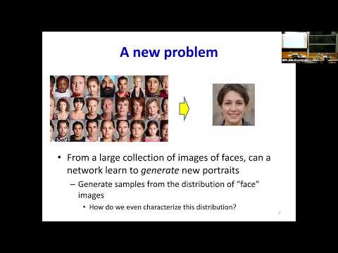
- The new goal is generative modeling: learn the distribution of faces or landscapes and sample new examples, rather than map labeled inputs to outputs.
- A 1000 by 1000 image can be represented as a million-dimensional point, but landscape images occupy only a restricted region of that space.
- Structure eliminates possible images, and probability density varies even within the region occupied by plausible data.
- A manifold approximates the shape of that region; generating examples also requires modeling probability density along it.
- A function mapping k-dimensional inputs to higher-dimensional outputs cannot fill the entire output space; its image is at most k-dimensional.
- A linear two-to-three-dimensional mapping produces a plane, while a nonlinear mapping can bend and fold that plane into a curved surface.
- The generative model can therefore represent data structure as a warped low-dimensional manifold embedded in pixel space.
- The decoder maps a latent input through a learned function to the data-space manifold, analogous to PCA's fitted plane but with nonlinear bending.
- Feeding latent values to the decoder can produce points on the learned surface, placing outputs in a more plausible region than arbitrary pixel-space samples.
- A basic decoder alone does not ensure that sampled latent points correspond to the training examples of interest.
- In the spiral example, increasing the one-dimensional latent value did not trace the spiral smoothly; the decoder jumped between data regions.
- Training data leave gaps in latent space, so an unconstrained decoder can behave unpredictably in those gaps.
- Sampling an arbitrary latent value may consequently produce an implausible output, such as a non-face when training on faces.
- The proposed remedy is to require latent codes to follow a continuous standard Gaussian distribution.
- A connected prior discourages the fragmented latent regions seen in the spiral example and gives sampling a defined, coherent region.
- The decoder still maps latent points onto a low-dimensional manifold; the prior regularizes how the manifold is parameterized.
- For a zero-mean, unit-variance isotropic Gaussian in d dimensions, the log density includes a constant and a term proportional to negative one-half the squared latent norm.
- The objective can be expressed as reconstruction training plus a penalty that encourages encoded latents to match the standard Gaussian prior.
- The lecture motivates this constraint through Gaussian likelihood and KL divergence, while noting that a simple squared-norm penalty is an incomplete account of distribution matching.
- A decoder can stretch, shrink, rotate, and bend latent space, changing the density of samples along the resulting manifold.
- The Gaussian prior does not mean generated faces are distributed like a Gaussian in pixel space; the nonlinear decoder transforms that distribution.
- A learned map can allocate more latent area to dense data regions and less to sparse regions, much like stretching a marked sheet or balloon.
- A decoder from a lower-dimensional latent space cannot generate a full-dimensional pixel distribution by itself, so the model adds output noise.
- The lecture treats off-manifold variation as uncorrelated Gaussian noise and favors small variance so that the manifold captures as much structure as possible.
- A Gaussian is used as maximally unstructured noise for a given variance, leaving structured variation for the learned manifold.
- Generation proceeds by sampling latent z from a standard Gaussian, decoding it to a point on the manifold, then adding output noise.
- If each training example's z were known, decoder parameters and noise variance could be trained by maximizing the likelihood of observed data.
- In practice z is unknown, and output noise means one observation can be explained by multiple latent values.
- Instead of assigning each input a unique z, the encoder estimates a posterior distribution of latent values that could have generated that input.
- The posterior for one face occupies a localized region, while the aggregate codes across all faces are encouraged to follow the global Gaussian prior.
- The encoder is deterministic in its outputs: it predicts distribution parameters, from which a latent sample is drawn.
- Training seeks a posterior approximation that both assigns high likelihood to the observed input and remains compatible with the global latent prior.
- The exact conditional distribution of z given x is intractable, so the model uses a tractable approximation and penalizes its KL divergence from the prior.
- Averaging this objective over training examples encourages aggregate latent codes to resemble a standard Gaussian.
- The encoder models the approximate posterior q(z given x) as a Gaussian, motivated by the locally near-linear behavior of a decoder with modest curvature.
- The encoder network predicts the Gaussian mean and variance for each input; a diagonal covariance is assumed for simpler computation.
- The Gaussian posterior is an approximation, not a claim that the true set of latent explanations for every input is exactly Gaussian.
- The decoder likelihood models x as Gaussian noise around the decoded point, with the output noise variance controlling the spread.
- To backpropagate through latent sampling, draw standard-normal epsilon and compute z as the encoder mean plus the standard deviation times epsilon.
- This reparameterization makes the sampled z differentiable with respect to the encoder's mean and variance parameters.
- The training objective combines reconstruction likelihood with a KL penalty between each approximate posterior and the standard Gaussian prior.
- The lecture interprets additional variance terms as accounting for uncertainty in z given x and for off-manifold output noise.
- After training, the decoder alone can generate examples by mapping samples from the standard Gaussian into data space.
- Examples show VAE samples resembling MNIST digits and human faces, with interpolations between latent means changing attributes such as neutral, smiling, and frowning expressions.
- Generated faces are often blurry because the model's Gaussian likelihood and limited decoder may average over structured alternatives rather than capture sharp detail.
- The lecture motivates hierarchical generative approaches: transform distributions in stages, an idea connected to latent diffusion models discussed in the next class.
Transcript excerpt
0:06 That's about it. And then I usually like for him I usually keep it at a wide shot so you can see the slides a nice shot but then zoom in when but then zoom in when he's writing on the board. >> Again like with the recitation they usually don't keep the board. You probably just keep it >> scares me. Te has those converters on top of the I think they're >> stabilizer. Yeah, the NDI. Are those that NDX encoder? NX. No, you're good.
0:58 >> Yeah, I got it. >> No problem. >> All right, there you go. You should be all set. >> Thank you very much. Yeah, they they have the microphone >> pretty well. >> Oh. Oh. Byebye. right here. >> How's it going?
2:19 orange Good. >> Yeah. combination. >> Yeah. Couple
3:23 extra Those are good. That's
6:23 Okay, good morning everybody. My machine's been crashing since last night. So, ah, it's nice to look up and actually see faces. And you've gone over there. >> Yeah. Anyways, uh we're going to start a new series of topics for the next uh four lectures. This is actually a continuation of what we did in the last class. What was the last topic we covered? >> Autoenccoder. What did we learn at the end of the class? What does the autoenccoder learn? >> Is that what the autoenccoder learned?
7:17 >> It's been two days. So, somebody has to give me the correct answer. What did the autoenccoder learn? small >> small representation but what else did it learn >> principle but was it pl is it was it linear >> so what exactly did the autoenccoder learn >> nonlinear features >> is it a nonlinear representation of features or is there was there a little more
This is the start of the transcript. Save this video free for the whole transcript, searchable and time-coded.
In this course
Related notes
Summary, takeaways, and chapters were generated by AI from the video's transcript and may contain errors. The video belongs to its creator, Carnegie Mellon University Deep Learning.