CMU Introduction To Deep Learning 11-785, Fall 2026: Lecture 21
Overview
The lecture explains neural-network classification as statistical estimation: cross-entropy training performs maximum-likelihood learning of class probabilities, while hidden layers transform inputs into features a final linear classifier can separate. It then interprets perceptron weights as learned pattern templates and connects autoencoders to PCA, nonlinear data manifolds, and source-specific decoders for generating and separating signals.
Key takeaways
- For binary classification, minimizing cross-entropy is maximum-likelihood estimation of P(Y|X), so the network learns calibrated class probabilities rather than only hard labels.
- A classification MLP can be understood as a feature extractor followed by a linear classifier: hidden layers reshape the representation until the output classes are linearly separable or nearly so.
- A perceptron's weight vector can be interpreted as a pattern template because its inner-product threshold responds to inputs sufficiently aligned with that vector.
- A linear autoencoder trained with squared reconstruction error recovers a principal subspace, while a nonlinear bottleneck decoder can represent a curved low-dimensional data manifold.
- A decoder trained on a source is constrained by its learned output manifold, which enables source-like generation and can support separating mixed signals by optimizing the latent inputs to multiple pre-trained decoders.
Chapters
- The opening minutes contain informal classroom conversation and brief exchanges before the lecture begins.
- The course moves into its scheduled lecture after attendance and classroom setup.
- The class focuses on what happens inside neural networks, beyond their external predictions.
- The lecture recaps neural networks as universal approximators, with CNNs for spatial patterns and LSTMs, GRUs, and transformers for time series.
- Students are asked to flag confusing explanations so the instructor can adjust the course.
- A linear classifier separates classes with a hyperplane, which is a line in the lecture's two-dimensional example.
- With overlapping or mislabeled data, no boundary perfectly separates the classes, so fitting every training point can produce an undesirable model.
- For 100 examples at the same input value, including 90 positive labels and 10 negative labels, a probability of 0.9 preserves more information than a hard label of 1.
- The lecture estimates the probability of a positive class by counting label frequencies in a neighborhood around each input.
- Sliding the neighborhood across a one-dimensional input produces a smooth estimate resembling a sigmoid.
- Tiny perturbations to input values show why a model should capture underlying class probabilities rather than memorize individual examples.
- A sigmoid neuron computes 1 / (1 + exp(-(w0 + w1x))), interpreted as P(Y=1|X=x).
- The sigmoid approaches 0 for large negative inputs and 1 for large positive inputs, while remaining differentiable.
- In multiple dimensions, the sigmoid forms a smooth surface; thresholding its output at 0.5 still gives a linear decision boundary.
- With labels encoded as +1 and -1, the logistic model assigns probability 1 / (1 + exp(-y z)), where z is the affine score.
- Assuming independent training examples, the likelihood of the dataset is the product of their conditional label probabilities.
- Maximizing the log-likelihood is equivalent to minimizing negative log-likelihood, which gives the classification cross-entropy objective.
- Cross-entropy training therefore estimates a statistical model of P(Y|X), rather than merely fitting arbitrary output values.
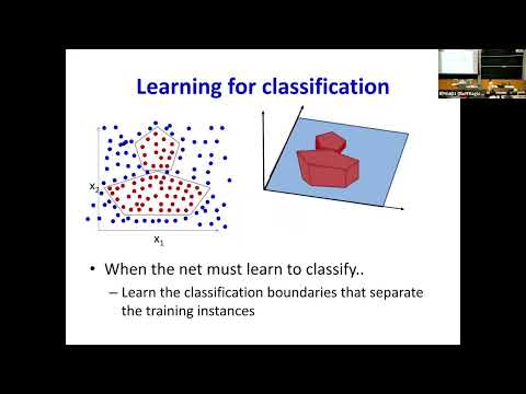
- A network can represent a double-pentagon decision region using hidden sub-networks for each pentagon and a final combining unit.
- The final sigmoid layer is a linear classifier in its input features, so the preceding network must transform the data into a linearly separable representation.
- If the hidden network has insufficient capacity, such as nine rather than ten required neurons in the example, it still seeks a useful separation but may not achieve the exact boundary.
- A trained penultimate representation can be paired with a different linear classifier, such as a support vector machine.
- The layers before the output form a feature extractor; the final layer uses a linear rule over those features.
- For overlapping classes, the output layer estimates P(Y|F(X)), where F(X) is the representation produced by the hidden network.
- The lecture emphasizes that limited model capacity does not guarantee which patterns gradient descent will learn; optimization may settle at different local minima.
- The manifold hypothesis frames complex data as lying on a nonlinear surface where classes may become separable after transformation.
- The network is described as progressively straightening or reshaping that data manifold across layers.
- A one-hidden-layer circle-classification example illustrates how affine transformations and nonlinear activations can transform nonlinearly separated data.
- The example maps two-dimensional inputs into three dimensions, where the affine layer places the data on a plane.
- A tanh activation bends that plane into a curved surface, and a later 3-to-1 affine projection collapses it onto a line.
- If the transformation succeeds, blue and red examples land on opposite sides of a one-dimensional threshold, yielding a circular boundary in the original input space.
- The training animation shows weights changing the plane and projection; optimization can pass through a good boundary and later worsen it.
- An 11-layer network trained on CIFAR-10 is visualized by projecting its layer representations into two or three dimensions with PCA.
- Class clusters become progressively more distinct through the network, and can become linearly separable before the final layers.
- Later layers may increase the gaps between already separable classes, improving robustness rather than creating separability from scratch.
- A perceptron computes the inner product between input vector X and weight vector W, then compares the score with a threshold.
- In high-dimensional spaces, the lecture notes that random vectors tend to lie near a sphere's surface, making inner-product thresholds interpretable through the angle between vectors.
- Under that view, a perceptron's weights encode a template: inputs sufficiently aligned with W activate the unit.
- For a grid-based digit example, weights drawn in the shape of a digit 2 would respond to inputs that correlate sufficiently with that pattern.
- First-layer perceptron weights can be inspected to see the patterns that units have learned to detect.
- A visualization that redraws each fired unit's weight pattern reveals which parts of a digit contributed to its classification.
- This reconstruction is selective rather than exact because a digit classifier retains task-relevant features and discards other input details.
- Training a network to reconstruct its input directly leads to the autoencoder setup.
- An autoencoder has an encoder that computes a hidden representation and a decoder that reconstructs the input.
- For the lecture's linear, tied-weight example, the encoder computes WX and the decoder returns WᵀWX while minimizing squared reconstruction error.
- With one hidden direction, outputs lie on the line spanned by W; with multiple hidden units, the corresponding reconstruction lies in a principal subspace.
- The lecture connects this linear reconstruction objective to principal component analysis.
- A linear decoder maps representations onto a linear subspace, while nonlinear decoder activations can bend that subspace into a curved surface.
- A bottleneck autoencoder therefore learns a low-dimensional manifold that approximates the structure of its training data.
- Because the decoder maps latent inputs onto its learned surface, its reconstructions are constrained to that surface rather than filling the entire output space.
- A network with a one-neuron bottleneck reconstructs two-dimensional spiral data along a learned one-dimensional helix-like manifold.
- Reconstruction is less accurate in regions without training examples, while observed portions of the spiral are captured more closely.
- A separate sinusoidal example illustrates how a nonlinear autoencoder can learn a curved data structure that linear PCA cannot represent directly.
- A decoder trained on digits or instrument recordings tends to generate outputs that resemble the training domain because its outputs lie on a learned data manifold.
- Separate autoencoders can be trained on different sound sources, such as guitar and drums, with only their decoders retained for signal separation.
- Backpropagation adjusts the latent inputs to the pre-trained decoders so their summed outputs match a mixed recording; the lecture demonstrates separation of string and wind instruments.
- The closing recap describes nonlinear autoencoders as learning a principal manifold and their decoders as source-specific generators.
Transcript excerpt
0:11 Okay. Yes. Let's go and study after this class. I'm just watching.
1:00 >> Look at him. >> I always make I have a deadline for something. >> [laughter] >> Oh,
1:48 no. >> KBKI. This is what exactly is current and so it's talking about >> I haven't seen this math. So on Friday at 2:00 we had a recession on different subject and after this this class was there and he was also master student and he was amazing at teaching like he was actually he was just so good. I got to learn from the end of the day. [snorts]
2:50 Okay. Give it to me. Happy. Sit down. [clears throat] >> That's good. >> Two days. What do you mean like Okay. >> Yeah. That's a good idea. >> Morning.
3:51 >> There's nothing deep about today's class. I'm just calling it neural networks. Haven't we done this? >> Good morning, professor. How are you? >> Good to see you, too. >> You're supposed to come here. >> I'm not going all the way back. >> See, [laughter] you can't say no. >> My kids and [laughter] Morning Lucas. That's cold.
4:57 Freezing. I was like, my hands are numb. But I walk. >> It's not cold. >> I'm I'm a weenie. >> We got another 20° to go south. >> I know. I got more layers to putus. >> Like two Januaries ago, it went to minus 40 with wind near our home. Our home fell apart. It cost us almost a quart million to fix it. >> - 40 is brutal. >> 24 radiators burst in our house. >> Think you're replaced with radiators, too? >> Like we couldn't because it's a 100-y old house. >> Yeah. >> So, large portions of our house are not heated right now.
This is the start of the transcript. Save this video free for the whole transcript, searchable and time-coded.
In this course
Related notes
Summary, takeaways, and chapters were generated by AI from the video's transcript and may contain errors. The video belongs to its creator, Carnegie Mellon University Deep Learning.