CMU Introduction To Deep Learning 11-785, Fall 2026: Lecture 23
Overview
The lecture develops diffusion models as a way to generate data by learning to reverse a fixed Gaussian-noising process, using a simple noise-prediction MSE objective rather than directly modeling the full data distribution. It connects DDPM training to score matching and reverse SDEs, explains how DDIM accelerates sampling, and covers classifier-free guidance, evaluation metrics, latent diffusion, ControlNet, DreamBooth, and video generation.
Key takeaways
- DDPM training avoids learning an intractable reverse distribution directly: it samples a clean image and noise level, adds known Gaussian noise in closed form, and trains a network with noise-prediction MSE.
- Log-uniform sampling across noise scales helps a model learn both global structure at high noise and fine image detail at low noise.
- DDIM accelerates generation by anchoring updates to a predicted clean sample, allowing large timestep skips; its zero-stochasticity setting makes sampling deterministic.
- Noise prediction and score estimation are connected: the learned direction points samples toward high-density regions of the data distribution and supports a reverse-SDE interpretation.
- Classifier-free guidance trains conditional and unconditional behavior in one model by dropping conditions on roughly 10 to 20% of training examples, then extrapolates toward the conditional prediction at inference.
- Latent diffusion reduces computational cost by denoising compressed representations, such as a 64×64×4 latent for a 512×512 image, while ControlNet and DreamBooth add structural and subject-specific control.
Chapters
- The lecture roadmap covers diffusion fundamentals, DDIM sampling, score matching, SDEs, classifier-free guidance, evaluation, and applications.
- The opening frames diffusion as a major approach to generative AI and previews both its mathematical foundations and practical uses.
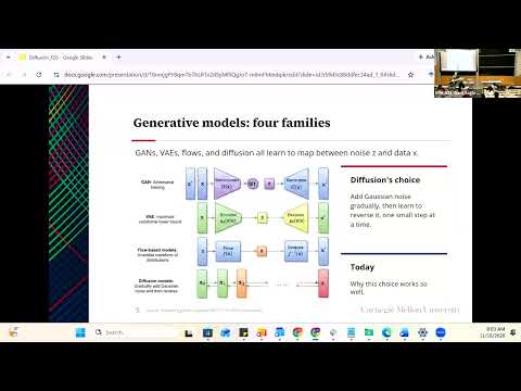
- Discriminative models estimate P(Y|X), while generative models aim to represent the data distribution P(X).
- GANs use a generator and discriminator but can suffer from unstable training and mode collapse.
- VAEs use an encoder and decoder but often produce blurry samples; flow models offer exact likelihoods but require invertible architectures.
- Diffusion models transform data through a chain of noise levels and learn to reverse that chain.
- A VAE decoder must bridge the gap from a simple latent distribution to a complex image in one pass, which can cause it to average details and produce blur.
- Diffusion replaces that single large jump with hundreds or thousands of smaller denoising steps.
- Diffusion resembles a hierarchical VAE, but its latent states have image dimensions, its forward noising process is fixed, and the learned component is the reverse process.
- The forward process is illustrated as Brownian motion: a concentrated ink drop spreads until its structure is lost in noise.
- Sohl-Dickstein et al. established the diffusion approach in 2015; Ho et al.'s 2020 DDPM formulation made it practical for image generation.
- DDPM trains a network to predict the Gaussian noise added to an image, rather than learning the reverse transition directly.
- The forward process is a Markov chain: each noisy state depends only on the immediately preceding state.
- Gaussian noise composition yields a closed-form way to sample a chosen noise level directly from the clean image, avoiding sequentially simulating every prior step.
- A variance schedule controls how much noise is added at each step, gradually transforming an image toward a standard Gaussian.
- The true reverse transition is intractable because it depends on the unknown data distribution, so a neural network approximates it.
- Training samples a clean image, a noise level, and Gaussian noise, then asks the model to predict that known noise.
- Mean squared error between predicted and actual noise provides a simple regression objective across images and noise levels.
- The lecture describes training across noise scales from approximately σ=0.01 to σ=100, with many discrete levels.
- Sampling σ uniformly in log space gives low- and high-noise ranges balanced attention; linear sampling would overemphasize extremely noisy examples.
- The training loop samples an image, timestep, and Gaussian noise, constructs the noisy input using the closed-form equation, and minimizes noise-prediction MSE.
- A 2D spiral dataset demonstrates diffusion with a simple MLP instead of an image-scale U-Net or transformer.
- The network receives noisy coordinates and a sinusoidal noise-level embedding, similar in purpose to transformer positional encodings.
- At high noise, predicted vectors point toward the distribution's broad center; at moderate noise they begin to follow the spiral, and at low noise they point toward nearby manifold points.
- The optimal noise predictor can be understood as a weighted average of training examples, with σ controlling how locally or broadly the model considers them.
- Low noise produces a nearest-neighbor-like, precise direction, while high noise averages over more examples and captures global structure.
- Adding noise smooths sharp, nondifferentiable geometry around the data manifold, making its gradient easier for a neural network to learn.
- The model shares parameters across noise levels and receives the noise-level embedding so it can apply the appropriate denoising behavior at each step.
- Standard DDPM generation begins with Gaussian noise and applies sequential denoising updates, often requiring hundreds or thousands of model evaluations.
- DDIM uses the predicted clean sample as an anchor and constructs updates that can skip large sections of the timestep schedule.
- With the stochasticity parameter set to zero, DDIM sampling is deterministic: the same starting noise produces the same output.
- Using around 50 DDIM steps instead of roughly 1,000 can substantially speed sampling while retaining comparable quality.
- The lecture recasts discrete noise steps as a continuous-time process described by stochastic calculus.
- An ordinary differential equation gives a deterministic path between noise and data distributions, while a stochastic differential equation adds a Brownian diffusion term.
- Both formulations describe transformations from a simple Gaussian prior toward the data distribution, with or without stochasticity.
- The score is ∇x log p(x), a direction toward higher-density regions that can be computed without knowing the distribution's normalizing constant.
- Predicting the added noise is mathematically related to estimating the score of the noisy data distribution.
- The learned score modifies the reverse SDE drift so samples are guided toward high-probability data regions rather than merely following an unguided random trajectory.
- Conditional generation changes the target from P(X) to P(X|Y), allowing labels or text prompts to steer samples toward a desired subset of data.
- Classifier guidance uses a separate noise-robust classifier; classifier-free guidance instead trains one model for conditional and unconditional prediction.
- During classifier-free guidance training, the condition is dropped about 10 to 20% of the time so the model learns both prediction modes.
- At inference, guidance extrapolates from the unconditional prediction toward the conditional prediction; increasing the guidance scale strengthens prompt adherence but sharpens the effective distribution.
- Fréchet Inception Distance (FID) compares generated and real image distributions in feature space, with lower scores indicating better alignment.
- Inception Score (IS) assesses image clarity and diversity, including whether samples avoid collapsing to repeated examples.
- Precision measures whether generated images look realistic, while recall measures how broadly the model covers the dataset.
- Latent diffusion runs denoising in a compact VAE representation rather than directly over every image pixel.
- A 512×512 image can be encoded into a 64×64×4 latent, reducing computation and allowing the model to focus on perceptually meaningful structure.
- Stable Diffusion uses an encoder, a denoising U-Net in latent space, and a decoder to reconstruct a high-resolution image.
- The VAE may discard fine detail, but its role is to provide a compact latent representation; the diffusion model performs the generative work.
- ControlNet adds a parallel network that uses structural inputs such as edge maps, depth maps, and pose skeletons to control image layout.
- DreamBooth fine-tunes a small part of a pretrained model using roughly three to five subject photos and associates the subject with a rare token.
- Video diffusion extends image diffusion across space and time; models such as Sora and Wan must preserve temporal consistency across frames.
- The closing principles are that many small denoising steps beat one large jump, the forward process is fixed while the reverse is learned, and denoising, score estimation, and reverse SDEs describe related views of the same model.
Transcript excerpt
1:49 I want you to stand with guidance on >> [snorts] [clears throat] >> Okay. So let's start.
3:22 Good morning everyone. Today we're going to explore one of the most exciting developments in generative AI which is diffusion model. So here is our roadmap for today. So we'll start by defining what's diffusion. We will explain the the process step by step. We'll look at the generation and the inference. What is DDIM? Then after that we will start exploring SDEs and score matching. We will also be talking about a classifier free guidance which gives us control on what to generate. Finally we will be um covering the evaluation and the real world applications. So, [snorts] to understand diffusion, we first have to ask, what's the goal of
4:11 the model? So, we have discriminative models [clears throat] which actually learn a mapping from an input to a label Y from input X to label Y. Essentially, we're learning a decision boundary. So, you can ask, is this a cat or a dog? But generative models, they're doing something much harder. They're not looking for a boundary. They're trying to learn the entire probability distribution of the data. So, they want to understand the essence of a cat so well that they can draw a brand new one from scratch. So, technically, we're moving from computing P Y given X to modeling the data distribution which is PX.
4:59 So, what does it mean to learn to generate data? So, how do we learn a distribution? Imagine every cat in our training set is a point in high dimensional space. These points, they cluster together on what we call the data manifold. So, the goal of generative um model is to take a simple, easy to sample distribution like Gaussian noise and
This is the start of the transcript. Save this video free for the whole transcript, searchable and time-coded.
In this course
Related notes
Summary, takeaways, and chapters were generated by AI from the video's transcript and may contain errors. The video belongs to its creator, Carnegie Mellon University Deep Learning.