CMU Introduction To Deep Learning 11-785, Fall 2026: Lecture 16
 Watch on YouTube →
Overview
CMU's 11-785 lecture develops Connectionist Temporal Classification (CTC) for sequence-to-sequence tasks whose outputs preserve order but lack timing alignments. It derives forward-backward posteriors to train over all valid alignments, introduces a blank symbol to distinguish repeated labels, and compares greedy decoding with beam search for finding likely output sequences.
Key takeaways
- CTC removes the need for frame-level alignment labels by summing over every valid alignment between an input sequence and its target output.
- The forward-backward algorithm computes each alignment node's posterior occupancy by combining forward and backward path probabilities, then normalizing across a time step.
- A blank symbol makes repeated labels representable: identical adjacent outputs collapse, but identical labels separated by a blank remain distinct.
- Greedy decoding finds the most likely time-synchronous path, which can differ from the most likely compressed sequence because that sequence's probability sums over many alignments.
- Beam search controls the exponential growth of candidate sequences by pruning to a top-K set, while equivalent prefixes must have their probabilities merged before ranking.
Chapters
- The opening minutes cover attendance, polling, and the instruction to close laptops and put phones away.
- At about 5:03, the lecture resumes sequence-to-sequence modeling, including speech recognition, machine translation, and dialogue.
- Input and output sequences may have different lengths; speech frames map to words without a one-to-one timing match.
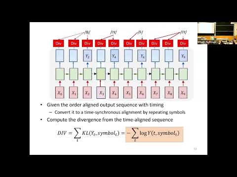
- When alignment labels are known, training can compare network output distributions with target symbols at each time step.
- For a fixed alignment, summing per-time negative log probabilities encourages the network to assign high probability to the target sequence.
- Viterbi training selects the highest-probability alignment, trains on it, then re-estimates alignments after updating the model.
- A poor initial alignment can yield a poor model and repeatedly reinforce bad alignments, trapping training in a local minimum.
- The lecture motivates considering the full distribution of possible alignments rather than committing to one path.
- Each valid path through the alignment graph has a probability, and the training objective can average divergence over paths using those probabilities as weights.
- The expectation of a sum can be rewritten as a sum of expectations, turning path-level loss into per-time, per-symbol contributions.
- The most probable Viterbi path is one alignment estimate, not ground-truth timing information.
- A graph node identifies a target symbol at a particular time; its posterior is the probability that a sampled alignment passes through it.
- The probability mass through a node factors into a forward probability for paths leading to it and a backward probability for paths leaving it.
- That factorization works because the network's output distribution at a time does not depend on which output symbol was sampled at the preceding time.
- The forward value alpha at a node sums the alpha values of its valid predecessor nodes, then multiplies by the current node's output probability.
- For the basic alignment graph, each node has at most two predecessors, such as staying on a target symbol or advancing to the next one.
- Initialization assigns the start node its output probability and unreachable nodes zero; the final alpha gives the total probability of the target sequence.
- The backward pass starts at the graph's final node and recursively sums valid successor probabilities, multiplying by the current node probability.
- Multiplying a node's forward and backward probabilities gives the mass of paths through that node; normalizing across a time column yields gamma, the node posterior.
- The expected divergence is computed by weighting each node's negative log output probability by gamma and summing over times and nodes.
- Symbols absent from the target alignment graph have zero loss contribution and zero derivative at that time.
- For a symbol appearing at multiple graph nodes in one time column, its posterior occupancies are summed; the lecture gives the output-probability derivative as the negative summed occupancy divided by that symbol's probability.
- The resulting per-time output derivatives are backpropagated through the network, typically a multilayer LSTM.
- For each training example, the procedure runs the network, extracts target-symbol probability rows, builds an alignment graph, and computes alpha, beta, and gamma values.
- Posterior-based output gradients are then propagated through the network to update its parameters.
- The forward-backward graph computation is presented as a small dynamic-programming operation, with work comparable to a forward and backward pass over the alignment graph.
- Without a separator, a time sequence such as repeated r and e outputs cannot distinguish the word “red” from “read.”
- CTC adds a blank symbol to the output vocabulary; adjacent repeated labels collapse, while a blank between them preserves two separate occurrences.
- For example, repeated r, blank, repeated e, blank, repeated d collapses to “red,” while repeated r, e, repeated e, d can collapse to “reed.”
- The target sequence is expanded into a graph that allows blank symbols between labels without requiring blank timing annotations in the training data.
- Adjacent identical target labels require a blank between them; otherwise the repeated outputs would collapse into a single label.
- For distinct neighboring labels, paths can advance directly or pass through a blank, representing multiple time-synchronous paths that map to the same target.
- The expanded graph permits initial and final blanks, so the forward pass initializes both permitted starting nodes and the backward pass initializes both permitted ending nodes.
- A node sums over its valid predecessors or successors; a skip across an intervening node is allowed only when the neighboring target symbols differ.
- After computing alpha and beta on the blank-extended graph, the same gamma and gradient procedure trains the network.
- Greedy decoding selects the most probable symbol at each time and then applies CTC collapsing, including blank removal and merging repeated labels.
- The resulting best time-synchronous path is not necessarily the most probable compressed output sequence.
- The lecture's “red” versus “Ted” example shows how one high-probability alignment can make greedy decoding prefer an output whose total probability across alignments is lower.
- The decoding objective is to find the compressed output sequence with the highest probability given the input, not merely the best individual time path.
- For a fixed candidate sequence, the forward algorithm's final alpha sums the probabilities of all alignments that collapse to it.
- Scoring every possible output sequence is computationally infeasible because the number of candidates grows exponentially.
- With labels S1 and S2 plus blank, the lecture organizes possible output strings and blank-separated extensions in a semi-tree.
- Unrolling the semi-tree across input time creates a graph where each row tracks alignments associated with an output prefix.
- A forward pass can score candidate sequences, but the graph grows exponentially as more input time steps are added.
- Beam search limits growth by retaining only the top K candidates at each step; the lecture uses top four as an example.
- Pruning keeps decoding tractable and can approach better solutions than greedy decoding as beam width increases.
- Candidates with the same compressed sequence, including versions ending in a blank or a label, must have their probabilities combined before ranking output sequences.
- The lecture summarizes CTC training as optimization over all valid alignments, with blanks separating repeated labels.
- Decoding options include greedy best-path decoding and beam search over candidate output sequences using forward probabilities.
- The next course section will remove the assumption that input and output sequences preserve order.
Transcript excerpt
1:59 Mhm. >> [clears throat]
3:28 [snorts] >> So guys, everybody in the attendance poll has 571. Please stand up. >> Check, check.
4:32 Wait, this is not how it's supposed to show up. Perfect. Okay, everybody. Usual stuff, laptops shut. Phones down. And let's begin. So, uh someone remind me what was the last we discussing? Anshu? We have to solve this problem of not or having alignment. The topic we are about was sequence-to-sequence modeling,
5:22 where the problem is that some the problem is conversion of one sequence to another. A some sequence of some length n goes in and a dick different sequence of some other length comes out. So, speech recognition, speech goes in, word sequence comes out. Machine translation, one word sequence goes in, a different word sequence comes out. And, you know, dialogue, you ask a question, the machine gives you an answer. All of these are sequence-to-sequence conversion problems. And amazingly enough, these are just functions, and amazingly enough, a neural network can do this. Now, there's no need for us to believe that there's any correspondence between the length or the word order of the input and the output or the uh or
6:08 what word and the order of the inputs. In some problems, there is a one-to-one correspondence correspond- corresponding to each input, there's an output. In other problems, there might be an order correspondence like in speech recognition. On the other hand, if you had machine translation, depending on how you write it, uh you know, the input and the output uh can have can mean the same thing, but the word orders could be entirely different. They could uh even be completely different things, right? My screen is blank, and the computer responds with please check if your computer is plugged in. So,
This is the start of the transcript. Save this video free for the whole transcript, searchable and time-coded.
Related notes
Summary, takeaways, and chapters were generated by AI from the video's transcript and may contain errors. The video belongs to its creator, Carnegie Mellon University Deep Learning.