CMU Introduction To Deep Learning 11-785, Fall 2026: Lecture 15
 Watch on YouTube →
Overview
CMU Lecture 15 builds from familiar sequence losses to the harder problem of training recurrent neural networks when input and output sequences have different lengths and their alignment is unknown. It formulates candidate alignments as paths through a probability graph, derives Viterbi decoding to select the most probable alignment in O(TM) time, and uses that alignment for a hard, iterative training procedure, while previewing Connectionist Temporal Classification (CTC) as a way to avoid committing to one alignment.
Key takeaways
- When every input has a matching output, sequence loss decomposes into a sum of local losses, making standard cross-entropy training straightforward.
- Intermittent sequence labels require alignment information: a transcript such as “good morning” does not specify the input timestamps for either word.
- Viterbi decoding finds the highest-probability target-preserving alignment with dynamic programming in O(TM) time instead of enumerating exponentially many paths.
- Greedy per-time-step decoding is not generally optimal because it ignores alternative paths and can collapse repeated symbols into one.
- Hard alignment training alternates between model updates and Viterbi realignment, but poor initialization can reinforce incorrect alignments and trap training in a local minimum.
- CTC is introduced as the next step because it can train without committing to a single explicit alignment and can distinguish repeated symbols using a blank separator.
Chapters
- The class resumes after fall break and introduces recurrent neural network sequence modeling.
- The lecture focuses on sequence-to-sequence tasks, where both inputs and outputs are sequences.
- The lecture distinguishes time-synchronous models, with one output per input, from sequence classification, which produces one label after a full sequence.
- Order-synchronous, time-asynchronous tasks produce intermittent outputs whose order follows the input, while sequence-to-sequence generation maps one whole sequence to another.
- A conventional MLP processes each input independently, so it has no recurrence or dependence on neighboring time steps.
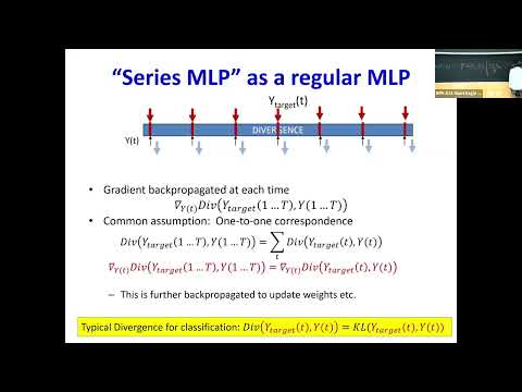
- When outputs correspond one-to-one with inputs, a sequence divergence can be written as a sum of per-time-step divergences, optionally weighted by time.
- Time-synchronous RNNs produce one output for every input, whether the network is unidirectional or bidirectional.
- Training commonly sums local KL divergences, equivalently cross-entropy losses, across time so gradients can be computed for each output.
- Sentiment classification and speech recognition can produce a single final label after processing the entire input sequence.
- Instead of training only on the final output, intermediate outputs can also receive labels, such as assigning the phoneme /ah/ throughout a sustained sound.
- Time-step weights can reflect where evidence appears, such as a sentiment becoming clear only when the word “glad” occurs.
- In speech recognition, words or phonemes occur intermittently, but the input does not specify their boundaries in advance.
- An RNN produces a probability distribution over the vocabulary at every time step, so decoding must determine which outputs to read and which to ignore.
- Maximum a posteriori classification selects the highest-probability class, and sequence decoding seeks the most probable output sequence given the input.
- A greedy method that picks the top symbol at every time and merges consecutive repeats can confuse an extended symbol with repeated symbols.
- Greedy choices also ignore alternative time alignments that may collectively give a target such as “yes” greater probability.
- A complete intermittent output specification includes both the symbol sequence and the time at which each symbol occurs.
- Those timestamps provide alignment, identifying which input regions correspond to target symbols, but ordinary speech transcripts do not include them.
- With a known alignment, each target symbol can be extended across its assigned input region and trained with a sum of per-time-step KL losses.
- Without timestamps, training must either guess an alignment or account for multiple possible alignments.
- The hard-alignment approach initializes timestamps, trains the model, uses its predictions to revise the alignment, and repeats.
- For the example target “beefy,” an initial guess assigns times to B, E, F, and the final E before model-based refinement.
- An asynchronous target such as “but” is a compressed sequence; repeating its symbols creates a time-synchronous expanded sequence aligned to the input.
- Many expanded sequences can compress to the same target, so alignment means finding the most probable valid expansion.
- The number of candidate alignments can be large even for a short target and a modest-length input.
- The RNN outputs a probability distribution over all vocabulary symbols at every time step.
- For a target such as “beefy,” selecting only its symbol rows prevents unrelated vocabulary items from entering a candidate alignment.
- Repeated target symbols, such as the two Es in “beefy,” appear as repeated rows in the restricted table.
- Choosing the most likely target symbol independently at each time can still produce symbols in the wrong order.
- The restricted table becomes a directed acyclic graph: paths move horizontally to repeat a symbol or diagonally downward to advance to the next target symbol.
- Every valid source-to-sink path represents an alignment that preserves the target sequence.
- A path score is the product of the RNN probabilities at all nodes visited along that path.
- Although the graph contains exponentially many complete paths, dynamic programming retains only the best path to each node.
- Viterbi decoding selects the best-scoring parent for each node, stores a backpointer, and multiplies the parent's path score by the current node probability.
- At the first time step, the source node receives its own probability as its path score; unreachable nodes receive score zero.
- For each later node, the algorithm compares its valid incoming parents, records the best parent, and updates the path score.
- Backtracking from the sink through stored parent pointers reconstructs the most probable alignment.
- For a graph with T input steps and M target rows, the lecture gives runtime proportional to T times M because each node has at most two candidate parents.
- The decoded path can differ from the locally most probable symbol in a time column if another choice yields a better complete target alignment.
- The result is a time-synchronous expansion of the original order-synchronous target.
- Treating the Viterbi path as the target alignment gives a per-time-step loss equal to the negative log probability assigned to the aligned symbol.
- The local loss derivative is zero for non-target symbols and equals negative one over the target probability for the target symbol.
- Backpropagation through these derivatives updates the RNN parameters using the selected alignment.
- The iterative procedure initializes alignments, trains the model, decodes updated alignments, and repeats; an SGD version can realign each example as training proceeds.
- Because it commits to one best alignment, the procedure is greedy and sensitive to poor initialization, which can lead to bad alignments and local minima.
- The next lecture will introduce CTC to train without explicit alignment, handle repeated symbols with a separator or blank, and improve inference.
Transcript excerpt
0:41 Are there other original names? >> The state of the paper how >> She's She She She's changed her name tag. Yeah. >> [laughter] >> Carbon dating the Yeah, it's not good enough. Uh exactly. >> [clears throat] >> My TA's are missing. Fall break
1:34 began on Monday and ended yesterday night, so it should be a Good morning. >> I'm ready. >> [clears throat]
3:09 >> So for the first time all semester long I'm beginning the class with how to single teaching assistant. >> [laughter] >> This is very lucky because for you guys because it means I don't get to call out Pokemons. I don't have my Pokemon names. >> Is there a chance to >> [laughter] >> I've had a few applications. So Who wants to be a TA? >> So it gets more work than being a student. >> There you go. I have a few. Okay. Perfect. >> This is this is called the battlefield promotion. >> [laughter] >> Thank you. It's good to see you. Yes. All right, folks. Your uh attendance poll is on the screen. Please
3:57 si- sign in. And we'll begin the second half of the semester, which uh I'm told is only 6 weeks long, at least 6 weeks of classes. So, you guys are [snorts] lucky. Yes. Aha. Yes. You have the Pokemons, right? So, I have a TA guys. I was just going to say my TA is okay. All right, let's begin. Uh the usual stuff, shut your laptops. Including those of you on Zoom. Good night. So, uh we're going to continue with our lectures on series on recurrent neural networks. Specifically, we are going to begin talking about sequence-to-sequence modeling.
4:44 If I say sequence-to-se- use the term sequence-to-sequence modeling, what does this term bring up to your minds?
This is the start of the transcript. Save this video free for the whole transcript, searchable and time-coded.
Related notes
Summary, takeaways, and chapters were generated by AI from the video's transcript and may contain errors. The video belongs to its creator, Carnegie Mellon University Deep Learning.