23. Differential Equations and exp(At)
Overview
Constant-coefficient linear systems u' = Au can be solved by finding A's eigenvalues and eigenvectors: each eigenmode evolves as e^(λt), and the initial condition determines how the modes combine. For A = [[-1, 2], [1, -2]] with u(0) = [1, 0], the solution combines a steady mode and an e^(-3t) mode, approaching [2/3, 1/3]; the lecture then defines e^(At) by its power series and derives e^(At) = S e^(Λt) S^(-1) when A is diagonalizable.
Key takeaways
- For u' = Au, every eigenpair (λ, x) gives a solution e^(λt)x, reducing the system to a combination of independent exponential modes when A is diagonalizable.
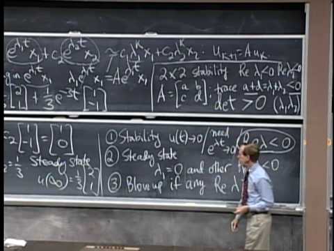
- For A = [[-1, 2], [1, -2]] and u(0) = [1, 0], the solution approaches [2/3, 1/3] because the λ = 0 mode remains while the λ = -3 mode decays.
- A continuous-time system is asymptotically stable exactly when all eigenvalues have negative real parts; complex imaginary components create oscillation but do not determine the decay rate.
- For a real 2×2 matrix, negative trace and positive determinant together characterize eigenvalues with negative real parts; negative trace alone does not rule out an unstable positive eigenvalue.
- The matrix exponential e^(At) = Σ(At)^n/n! converges for every finite A and t, and diagonalization yields the computational formula S e^(Λt) S^(-1).
- A kth-order scalar linear differential equation can be rewritten as a k-dimensional first-order system by using successive derivatives as state variables, enabling eigenvalue-based analysis.
Chapters
- The central problem is solving first-order systems of the form u' = Au, where A is a constant coefficient matrix.
- Each eigenvalue and eigenvector of A produces a pure exponential solution, connecting differential equations to matrix powers.
- For A = [[-1, 2], [1, -2]], the dependent columns make A singular, so one eigenvalue is 0.
- The trace is -3, so the other eigenvalue is -3; the characteristic polynomial is λ(λ + 3).
- The eigenvalue 0 signals a constant mode, while -3 produces a component that decays like e^(-3t).
- A nullspace vector for λ = 0 is [2, 1], satisfying A[2, 1] = 0.
- For λ = -3, [1, -1] is an eigenvector, satisfying A[1, -1] = -3[1, -1].
- The general solution is a linear combination of these vectors multiplied by e^(0t) and e^(-3t), respectively.
- With u(0) = [1, 0], matching the eigenvector combination gives coefficients c1 = c2 = 1/3.
- The solution is (1/3)[2, 1] + (1/3)e^(-3t)[1, -1].
- As t approaches infinity, the decaying mode vanishes and the state approaches [2/3, 1/3].
- A system decays to zero for every initial condition when every eigenvalue has negative real part.
- For λ = -3 + 6i, e^(λt) has magnitude e^(-3t): the imaginary part causes oscillation, while the real part controls decay.
- A zero eigenvalue with all other eigenvalues having negative real parts can produce a steady state; any positive real part causes growth.
- For a real 2×2 matrix, stable eigenvalues require negative trace, since trace equals the sum of the eigenvalues.
- Negative trace alone is insufficient: diag(-2, 1) has negative trace but its positive eigenvalue causes exponential growth.
- Negative trace and positive determinant together ensure both eigenvalues have negative real parts.
- Place the eigenvectors in the columns of S; the initial modal coefficients satisfy S c = u(0).
- Changing variables to u = Sv converts u' = Au into v' = Λv, where Λ is diagonal and each component evolves independently.
- The solution takes the form u(t) = S e^(Λt) S^(-1)u(0), defining e^(At) for a diagonalizable matrix.
- The matrix exponential is defined as I + At + (At)^2/2! + (At)^3/3! + continuing terms (At)^n/n!.
- The factorial denominators make the exponential series converge for every finite matrix A and time t.
- The geometric-series analogue I + At + (At)^2 + ... can represent (I - At)^(-1) when the eigenvalues of At have magnitude less than 1.
- Substituting A = SΛS^(-1) into each power of the exponential series gives A^n = SΛ^nS^(-1).
- Factoring out S and S^(-1) leaves e^(At) = S e^(Λt) S^(-1).
- This diagonalization formula requires a full set of independent eigenvectors; the power-series definition still applies when A is not diagonalizable.
- For diagonal Λ, e^(Λt) has entries e^(λ₁t), ..., e^(λₙt), so e^(At) decays when every eigenvalue has negative real part.
- Continuous-time stability requires eigenvalues in the left half of the complex plane; matrix powers decay when eigenvalues lie inside the unit circle.
- A second-order equation y'' + by' + Ky = 0 becomes a two-variable first-order system using the state [y', y] and a companion matrix with first row [-b, -K] and second row [1, 0].
Transcript excerpt
0:00 -- and lift-off on differential equations. So, this section is about how to solve a system of first order, first derivative, constant coefficient linear equations. And if we do it right, it turns directly into linear algebra. The key idea is the solutions to constant coefficient linear equations are exponentials. So if you look for an exponential, then all you have to find is what's up there in the exponent and what multiplies the exponential
0:51 and that's the linear algebra. So -- and the result -- one thing we will fine -- it's completely parallel to powers of a matrix. So the last lecture was about how would you compute A to the K or A to the 100? How do you compute high powers of a matrix? Now it's not powers anymore, but it's exponentials. That's the natural thing for differential equation. Okay. But can I begin with an example? And I'll just go through the mechanics. How would I solve the differential -- two differential equations? So I'm going to make it -- I'll have a two by two matrix and the coefficients are minus one two, one minus two and I'd better give you
1:42 some initial condition. So suppose it starts u at times zero -- this is u1, u2 -- let it -- let it -- suppose everything is in u1 at times zero. So -- at -- at the start, it's all in u1. But what happens as time goes on, du2/dt will -- will be positive, because of that u1 term, so flow will move into the u2 component and it will go out of the u1 component. So we'll just follow that movement as time goes forward by looking at the eigenvalues and eigenvectors of that matrix.
2:30 That's a first job. Before you do anything else, find the --
This is the start of the transcript. Save this video free for the whole transcript, searchable and time-coded.
Related notes
Summary, takeaways, and chapters were generated by AI from the video's transcript and may contain errors. The video belongs to its creator, MIT OpenCourseWare.