32. Quiz 3 Review

Overview

The review covers Chapter 6 topics for Quiz 3, including eigenvalue shortcuts, matrix exponentials, symmetric and skew-symmetric matrices, similarity, positive definiteness, and the singular value decomposition (SVD); Chapter 7 linear transformations are reserved for the final. Worked examples show how eigenvalues reveal the behavior of differential-equation solutions and matrix properties, while the SVD exposes rank and null spaces.

Key takeaways

For a real symmetric matrix, orthogonal diagonalization A = QΛQᵀ provides real eigenvalues and an orthonormal eigenbasis, including when eigenvalues repeat.
A skew-symmetric matrix has purely imaginary eigenvalues or zero; in the 3×3 example, eigenvalues 0 and ±√2 i produce bounded oscillations with period π√2.
For a diagonalizable matrix A = SΛS⁻¹, the matrix exponential is e^(At) = Se^(Λt)S⁻¹, so each eigenmode evolves as e^(λᵢt).
The SVD is available for rectangular as well as square matrices; the number of nonzero singular values gives the rank, and zero-singular-value right vectors span the null space.
Singular values are nonnegative, and the relation Avᵢ = σᵢuᵢ fixes the sign of each left singular vector after choosing the corresponding right singular vector.
A symmetric orthogonal matrix has eigenvalues only +1 and −1, making (A + I)/2 a symmetric idempotent projection.

Chapters

0:00 Chapter 6 Scope and the Key Facts About Matrix Classes

Quiz 3 covers through Chapter 6; Chapter 7 linear transformations are excluded and reserved for the final review.
A symmetric matrix has real eigenvalues and enough mutually orthogonal eigenvectors for a decomposition A = QΛQᵀ.
Similar matrices share eigenvalues, and their powers are related by Bᵏ = M⁻¹AᵏM.

4:40 Setting Up a Matrix Differential Equation and Finding a Zero Eigenvalue

For u′ = Au with a 3×3 matrix and no specified initial condition, the general solution combines three eigenvector modes with arbitrary constants.
The example matrix is singular because its first and third columns are linearly dependent, so zero is an eigenvalue.
Checking whether a matrix is singular can identify an eigenvalue before computing det(A − λI).

8:00 Skew-Symmetric Eigenvalues, Stability, and Periodic Solutions

The example satisfies Aᵀ = −A, so it is skew-symmetric and its eigenvalues are 0 and ±√2 i.
The modes e^(λt) have constant magnitude for the imaginary eigenvalues, so solutions neither decay to zero nor grow without bound.
The oscillatory modes return to their starting phase after T = 2π/√2 = π√2.

13:30 When Eigenvectors Are Orthogonal: The Commutator Test

A matrix has orthogonal eigenvectors when AAᵀ = AᵀA, meaning it commutes with its transpose.
Symmetric matrices satisfy the condition because Aᵀ = A; skew-symmetric matrices satisfy it because Aᵀ = −A.
Orthogonal matrices satisfy the condition because QQᵀ = QᵀQ = I.

16:20 Computing the Matrix Exponential for u′ = Au

The solution with initial value u(0) is u(t) = e^(At)u(0).
If A is diagonalizable as A = SΛS⁻¹, then e^(At) = Se^(Λt)S⁻¹.
The diagonal entries of e^(Λt) are e^(λᵢt), and the formula requires enough eigenvectors to diagonalize A.

18:20 Testing Diagonalizability, Definiteness, Markov Structure, and Projection

In the given 3×3 example, the stated eigenvectors are orthogonal and independent, so the matrix is diagonalizable for every value of c.
The matrix is symmetric when c is real; it cannot be positive definite because one eigenvalue is zero, though it is positive semidefinite when c ≥ 0.
It cannot be a Markov matrix because it has an eigenvalue 2, while Markov-matrix eigenvalues cannot exceed 1 in magnitude.
A/2 is a projection when c = 0 or c = 2, since projection eigenvalues must be 0 or 1.

25:50 SVD Construction from AᵀA and the Sign Rule for U

Every matrix, including rectangular matrices, has an SVD A = UΣVᵀ with orthogonal factors and nonnegative singular values.
The columns of V are eigenvectors of AᵀA, and the singular values σᵢ are the nonnegative square roots of its eigenvalues.
Eigenvectors of AAᵀ identify the columns of U only up to sign; use Avᵢ = σᵢuᵢ to determine each left singular vector consistently.

34:00 Reading Invertibility, Rank, and Null Spaces from the SVD

A 2×2 SVD with singular values 3 and 2 describes an invertible matrix because neither singular value is zero.
Singular values 3 and 0 indicate rank 1, so the 2×2 matrix has a one-dimensional null space.
For the zero singular value, the corresponding right singular vector v₂ lies in the null space of A; the SVD also reveals column-space and left-null-space information.

38:47 Symmetric Orthogonal Matrices and the Projection (A + I)/2

If A is both symmetric and orthogonal, its eigenvalues are real and have magnitude 1, so they can only be +1 or −1.
Such a matrix need not be positive definite and may have repeated eigenvalues, but it is orthogonally diagonalizable and nonsingular.
Because Aᵀ = A and A² = I, P = (A + I)/2 is symmetric and satisfies P² = P, making it a projection.
The eigenvalues of P are 0 and 1, obtained by shifting A's eigenvalues by 1 and dividing by 2.

Transcript excerpt

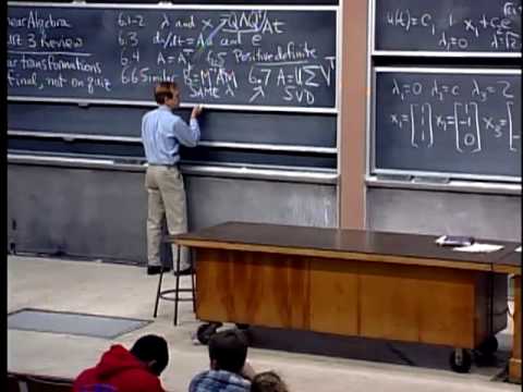
0:07 OK, here we go with, quiz review for the third quiz that's coming on Friday. So, one key point is that the quiz covers through chapter six. Chapter seven on linear transformations will appear on the final exam, but not on the quiz. So I won't review linear transformations today, but they'll come into the full course review on the very last lecture. So today, I'm reviewing chapter six, and I'm going to take some old exams, and I'm always ready to answer questions. And I thought, kind of help our memories if I write down the main topics in chapter six.

1:00 So, already, on the previous quiz, we knew how to find eigenvalues and eigenvectors. Well, we knew how to find them by that determinant of A minus lambda I equals zero. But, of course, there could be shortcuts. There could be, like, useful information about the eigenvalues that we can speed things up with. OK. Then, the new stuff starts out with a differential equation, so I'll do a problem. I'll do a differential equation problem first. What's special about symmetric matrices? Can we just say that in words? I'd better write it down, though.

1:48 What's special about symmetric matrices? Their eigenvalues are real. The eigenvalues of a symmetric matrix always come out real, and there always are enough eigenvectors. Even if there are repeated eigenvalues, there are enough eigenvectors, and we can choose those eigenvectors to be orthogonal. So if A equals A transposed, the big fact will be that we can diagonalize it, and those eigenvector matrix, with the eigenvectors in the column, can be an orthogonal matrix. So we get a Q lambda Q transpose. That, in three symbols, expresses a wonderful fact,

2:43 a fundamental fact for symmetric matrices. OK. Then, we went beyond that fact to ask

This is the start of the transcript. Save this video free for the whole transcript, searchable and time-coded.

Related notes

Summary, takeaways, and chapters were generated by AI from the video's transcript and may contain errors. The video belongs to its creator, MIT OpenCourseWare.