STAT 638 (Fall 2026), Lecture 35
Overview
Samiran Sinha uses the German DAX index to compare four Gaussian-process models for log stock prices: white noise around a linear trend, stationary AR(1), squared-exponential Gaussian process plus white noise, and Brownian motion. He explains their return and forecast-uncertainty behavior, fits them by maximum likelihood, and evaluates them with variance-ratio diagnostics, AIC, innovation checks, and chronological train, validation, and test splits; AR(1) has the lowest AIC, while AR(1) and Brownian motion emerge as leading forecast candidates.
Key takeaways
- Independent Gaussian noise added to a log-price trend produces consecutive daily log returns with correlation −0.5, because adjacent differences share one noise term.
- For Brownian-motion errors, an H-day log-price change has variance σB²H and standard deviation σB√H, so predictive uncertainty expands with the forecast horizon.
- The observed DAX variance ratios, 3.02, 5.46, and 17.779 at 3, 5, and 20 days, align reasonably well with Brownian-motion predictions of 3, 5, and 20.
- The fitted AR(1) model has φ = 0.9912, the lowest AIC, and variance ratios close to the observed values at all three evaluated horizons.
- Model evaluation for time series should preserve chronology: Sinha uses the first 70% of observations for training, the next 15% for validation, and the final 15% for testing.
- Forecast selection should assess both point accuracy and uncertainty calibration, using measures such as RMSE, mean negative log predictive density, and 95% prediction-interval coverage.
Chapters
- Each student is assigned one project to grade, with two or three graders assigned to each project for consistency.
- The rubric awards 0, 0.5, or 1 point per item, and graders should comment when deducting points.
- Sinha asks students to complete the course evaluation and begin grading their assigned project after the lecture.
- The example uses daily closing levels of Germany's DAX stock market index, with the modeled response defined as the log price, Lₜ = log(Pₜ).
- The forecasting goal is to predict the next trading day's closing level and quantify uncertainty at horizons of 1, 3, 5, and 20 trading days.
- Sinha starts with a linear trend, Lₜ = α + μt + Bₜ, and notes that polynomial trends could replace the linear component.
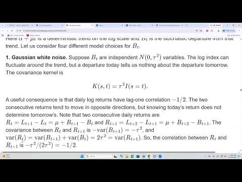
- In the first model, Bₜ is independent Gaussian white noise with variance τ², giving a diagonal covariance matrix for the noise vector.
- Although consecutive noise terms are independent, returns formed by differencing adjacent log prices share a noise term.
- The resulting lag-1 correlation between consecutive daily log returns is −0.5, so adjacent returns tend to move in opposite directions.
- The stationary Gaussian AR(1) model uses Bₜ = φBₜ₋₁ + εₜ, with |φ| < 1 and Gaussian innovations; positive φ makes shocks persist while their effects decay over time.
- The squared-exponential model represents Bₜ as a smooth zero-mean Gaussian process plus independent white noise, combining a radial-basis-function kernel with a noise term.
- The Brownian-motion model sets Bₜ = σB Wₜ, with covariance K(s,t) = σB² min(s,t); its consecutive Gaussian returns are independent.
- Under Brownian motion, an H-day log-price change has mean μH and variance σB²H, so its standard deviation grows as σB√H.
- Consecutive returns are uncorrelated under Brownian motion and, because they are jointly Gaussian, are independent.
- The four alternatives are all Gaussian processes on the observed time grid; their central difference is the covariance structure, not whether they qualify as Gaussian processes.
- Sinha compares the variance of an H-day log return with the variance of a one-day return, using theoretical ratios implied by each covariance model.
- For white noise around the trend, the ratio is 1 for every horizon; for Brownian motion, it is H.
- For stationary AR(1), the ratio depends on φ and approaches a finite limit as H grows, while the squared-exponential model has its own parameter-dependent pattern.
- The observed DAX variance ratios are 3.02 for 3-day returns, 5.46 for 5-day returns, and 17.779 for 20-day returns.
- Those values are fairly close to Brownian-motion predictions of 3, 5, and 20, especially at 3 and 5 days.
- For model evaluation, the series is split chronologically into 70% training data, 15% validation data, and 15% test data, rather than randomly shuffled.
- Sinha fits each model using its multivariate Gaussian likelihood and covariance matrix, optimizing the negative log-likelihood to estimate trend and covariance parameters.
- The parameter estimates include AR(1) φ = 0.9912 and Brownian-motion σB = 0.0092; the AR(1) coefficient indicates highly persistent dependence.
- AIC ranks AR(1) first and Brownian motion second, with white noise having the largest AIC among the four candidates.
- With fitted φ = 0.9912, AR(1) variance ratios are 2.97, 4.91, and 18.41 at horizons of 3, 5, and 20 days, respectively, close to the observed 3.02, 5.46, and 17.779.
- Model diagnostics examine standardized one-step prediction errors, their autocorrelations and squared-error autocorrelations, and normal QQ plots; dependence in the errors signals a poor white-noise assumption.
- Validation compares predictive distributions using mean negative log predictive density, RMSE, and 95% interval coverage; Brownian motion has the highest reported coverage, while AR(1) coverage is about 0.91.
- AR(1) and Brownian motion are retained as the leading candidates, then evaluated on the held-out test period with parameter estimates fixed; Brownian motion is also used as a benchmark.
- The forecast plots show median predictions and 95% prediction intervals for 1-, 3-, 5-, and 20-day horizons, with wider intervals at longer horizons.
- Sinha encourages applying the models to other indices or stocks, including Apple, Amazon, and NVIDIA, and says student presentations should last 8 to 10 minutes and use Zoom.
Transcript excerpt
0:01 Sinha, Samiran: Alright, so, let's get started. Sinha, Samiran: Before I start, few things about… Sinha, Samiran: about the email I sent during the weekend, is That now you can see… Who is going to grade? Sinha, Samiran: which project, right? So this is the project assignment with the grader's name. Sinha, Samiran: Everyone will be getting just one project, right? Sinha, Samiran: And every project will be graded by? Sinha, Samiran: Multiple people. Sinha, Samiran: 3 to 2 people, okay? Every project. Sinha, Samiran: So that is good, I think, for consistency, that we are getting, good number of graders.
0:56 Sinha, Samiran: Also, grading rubrics. This is very good. Sinha, Samiran: I have separated the points. It will be very easy for you guys to gradually look at that topic. Sinha, Samiran: If it is not addressed, Properly, then get 0.5. If it is addressed properly, one point. Sinha, Samiran: And if it is not addressed. Sinha, Samiran: at all, then zero points. So this is a very good thing, and then you add… add all the points. Sinha, Samiran: And get the total points. And if you take off some points, this is very important. Sinha, Samiran: If you take off some points. Sinha, Samiran: Then you write a comment beside that. Sinha, Samiran: This is what, very good thing in this country. When I moved here, from the country, where people used to give the positive marking, okay? But here, that shows you the negative marking and why it is negative. Sinha, Samiran: This is a very, good feedback, I think.
1:57 Sinha, Samiran: Okay, so this is… 8, and then course evaluation. Sinha, Samiran: So please fill up the course evaluation there. I will not be able to open it, but it is available here. Please do so, okay?
This is the start of the transcript. Save this video free for the whole transcript, searchable and time-coded.
In this course
Related notes
Summary, takeaways, and chapters were generated by AI from the video's transcript and may contain errors. The video belongs to its creator, Samiran Sinha.