STAT 638 (Fall 2026), Lecture 33
Overview
Samiran Sinha finishes an exam discussion using the anorexia data from R's MASS package, showing how MCMC estimates hierarchical treatment effects and posterior probabilities. He then introduces Gaussian processes, from Brownian motion and Brownian bridges to nonparametric regression, explaining how conditional multivariate normal distributions produce predictions and uncertainty estimates, and how kernel hyperparameters can be fitted by maximizing likelihood.
Key takeaways
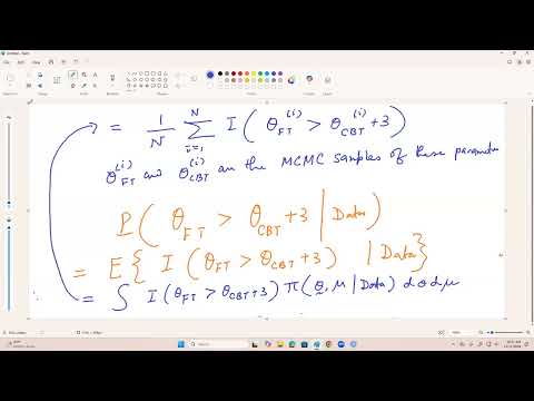
- For the anorexia example, averaging posterior indicators across 90,000 retained MCMC draws estimates the probability that the FT mean exceeds the CBT mean by more than 3 pounds; the estimate is about 0.73.
- Posterior prediction for a new FT patient must include both uncertainty in theta_FT and observation noise; with noise variance 25, the estimated chance of at least a 5-pound gain is about 0.647.
- A Gaussian process is defined by the requirement that every finite vector of process values is multivariate normal, with its covariance kernel specifying dependence across index points.
- Brownian motion has covariance min(s, t), variance delta for an increment of length delta, and independent non-overlapping increments; a Brownian bridge modifies the process so both endpoints are zero.
- Gaussian-process regression predicts an unobserved function value by conditioning a joint multivariate normal distribution, yielding both a predictive mean and a predictive variance.
- Gaussian-process predictions depend on kernel and noise hyperparameters, including length scale, signal variance, and observation-noise variance; maximum likelihood provides one approach to estimating them.
Chapters
- Samiran Sinha plans to complete the exam discussion before covering Gaussian processes as material beyond chapters 1 through 10.
- The lecture uses the exam's anorexia treatment data to revisit hierarchical modeling and MCMC.
- The example uses the anorexia dataset from R's MASS package, defining weight change as post-treatment weight minus pre-treatment weight.
- A hierarchical model estimates means for family treatment (FT), cognitive behavioral treatment (CBT), and control, along with a grand mean.
- Hierarchical modeling is especially useful when group samples are modest and vary in size, as in this dataset.
- After discarding 10,000 burn-in iterations, the estimated posterior mean weight change for FT is about 6.92 pounds.
- The target probability is that the FT population mean exceeds the CBT mean by more than 3 pounds, given the data.
- Sinha estimates it by averaging the indicator of theta_FT > theta_CBT + 3 across retained posterior draws.
- The estimated probability is about 0.73, or 73 percent.
- The chain has 100,000 draws; removing the first 10,000 burn-in draws leaves 90,000 indicators for the Monte Carlo estimate.
- For a new FT patient, the model writes weight change as the sampled group mean theta_FT plus observation noise.
- The noise is normally distributed with mean 0 and variance 25, equivalent to a standard deviation of 5 pounds.
- Sinha adds a simulated noise draw to each retained MCMC draw of theta_FT to form a posterior predictive sample.
- The estimated probability that the new patient's weight gain is at least 5 pounds is about 0.647.
- A Gaussian process is a collection of random variables indexed by a set T, with a mean function and covariance kernel.
- For any finite selection of index points, the corresponding vector of process values follows a multivariate normal distribution.
- The index set may be discrete or continuous, and a centered Gaussian process has mean zero at every index.
- Standard Brownian motion is indexed by time from 0 onward, has mean zero, and uses covariance kernel min(s, t).
- It starts at zero with probability 1, and an increment over an interval of length delta has variance delta.
- Consecutive non-overlapping increments, such as X(t + h) - X(t) and X(t + 2h) - X(t + h), are independent.
- Sinha notes applications in particle movement, spatial modeling, and financial stock-price modeling.
- A Brownian bridge is indexed over a bounded interval and is constrained to equal zero at both endpoints.
- Its covariance kernel adjusts the Brownian-motion kernel to enforce the endpoint constraint; a bridge can also be constructed from Brownian motion.
- Sinha illustrates a general Gaussian process on 100 points from 0 to 1 using a radial basis function (RBF) covariance kernel and a multivariate normal draw.
- The connected values form a sample path; unlike Brownian motion, a general RBF Gaussian process does not have independent consecutive increments.
- Classical regression assumes a specified mean form such as beta_0 + beta_1 x, while polynomial regression extends that form with powers of x.
- Gaussian-process regression instead models Y = F(x) + error, with normal noise of variance sigma squared and F assigned a Gaussian-process prior.
- The mean function is often set to zero or a constant, while the covariance kernel encodes dependence between function values at different inputs.
- The goal is to predict F(x_0) at an unobserved input and quantify uncertainty, such as estimating oil quality or depth between costly exploration sites.
- The observed responses and the unknown value F(x_0) have a joint multivariate normal distribution; conditioning on observed data gives the predictive mean and variance.
- Gaussian-process regression is nonparametric and provides both a point prediction and an uncertainty estimate, with smoothness controlled by the covariance kernel.
- Kernel parameters such as length scale eta, signal variance tau squared, and observation-noise variance sigma squared must be estimated from data.
- Sinha describes maximizing the multivariate-normal log likelihood to estimate these parameters, then plans to apply the method to zinc concentrations measured at different locations.
Transcript excerpt
0:15 Sinha, Samiran: So, today, we'll talk about… Two things. One, We'll complete the discussion. Sinha, Samiran: on the exam. Sinha, Samiran: And we'll start a new material. If you do not have any questions, then we can talk about Sinha, Samiran: A material on… Gaussian process. Sinha, Samiran: And this is something extra I'm doing. Beyond chapter 1 to 10, this is something extra. Sinha, Samiran: So, this is the dataset we have been talking, the dataset for our… Exam question.
2:44 Sinha, Samiran: So this is the dataset. Use the anorexia data. Sinha, Samiran: From the R-package mass, define the weight change as the post-treatment weight minus pre-treatment weight. Sinha, Samiran: And we have this hierarchical model. Sinha, Samiran: Okay? And, observations are independent, conditional on the group means, the variances are known. So, as you see in this dataset. Sinha, Samiran: The number of observations? Sinha, Samiran: Maddie? Sinha, Samiran: Across the groups. Sinha, Samiran: Right? So that is the reason we are doing hierarchical model. Hierarchical model will be useful Sinha, Samiran: If you have a small sample size for every group. Sinha, Samiran: And if you have a lot of variations in the sample sizes across the groups, then it is very useful. If the sample size for every group is very high, then it is not so useful.
3:49 Sinha, Samiran: So, in our case, the number of observations are… NCBT. Sinha, Samiran: is… 29? Sinha, Samiran: 26, and… Sinha, Samiran: 70, so there is quite a bit of variation in the sample sizes, and also the sample sizes are not large. So, in this case, it is worth considering this hierarchical model. Sinha, Samiran: And the question is, what is the posterior mean noise change for the family treatment group? So, we estimated, through MCMC mechanism, theta 1, theta 2, theta 3, 3 group means, corresponding to the treatment groups.
This is the start of the transcript. Save this video free for the whole transcript, searchable and time-coded.
In this course
Related notes
Summary, takeaways, and chapters were generated by AI from the video's transcript and may contain errors. The video belongs to its creator, Samiran Sinha.