Mathematical Foundations of AI Alignment Lecture 5.1 (Maximal Lotteries and No Regret Learning)

Overview

Aaron Roth connects preference aggregation to zero-sum game theory: majority cycles can make every deterministic completion vulnerable, while a randomized distribution can potentially tie or defeat every challenger. He defines maximal lotteries through a skew-symmetric preference-margin matrix, introduces von Neumann's minimax theorem, and proves the Hedge algorithm's no-regret guarantee, with regret at most ln(d)/η + ηT/2 and average regret shrinking at order 1/√T; the next lecture will use Hedge to complete the minimax proof and derive a method for finding maximal lotteries.

Key takeaways

In a cyclic preference population, no deterministic completion can be immune to an adaptive challenger, but randomization can eliminate the exploitable pure choice.
The pairwise margin matrix M is skew-symmetric, and a lottery P is maximal exactly when PᵀMQ ≥ 0 for every challenger distribution Q.
Von Neumann's minimax theorem says that mixed strategies make the maximin and minimax values equal in every finite zero-sum game, removing any disadvantage from moving first.
Hedge uses the update wₜ₊₁(a) = wₜ(a)exp(-ηℓₜ(a)) and guarantees regret at most ln(d)/η + ηT/2 for losses in [-1,1].
With an appropriate learning rate, Hedge's average regret decreases at order 1/√T, even against loss vectors chosen adaptively after observing its current mixed strategy.
The lecture establishes Hedge's regret bound and lays out, rather than completes, the repeated-play proof that will use no-regret learning to establish minimax and compute maximal lotteries.

Chapters

0:00 Preference Cycles Make Deterministic Completions Vulnerable

Three equally common preference types rank completions A, B, and C as A>B>C, B>C>A, and C>A>B.
Pairwise majorities cycle: two-thirds prefer A to B, B to C, and C to A.
A model that always outputs one completion can be challenged by another deterministic model that a majority prefers.

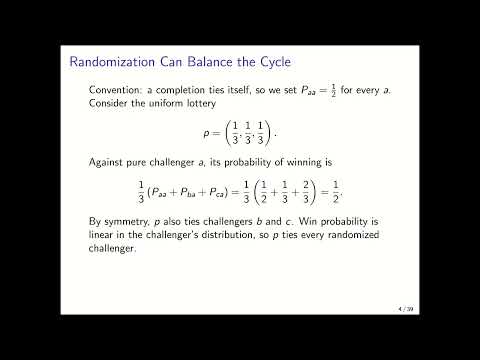
5:00 A Uniform Lottery Ties Every Pure Challenger

Randomizing uniformly over A, B, and C neutralizes the cyclic example's advantage for any single deterministic completion.
Against a challenger that always outputs A, the uniform policy ties on average after accounting for ties and the population's preferences.
Because expected comparisons are linear in the challenger's distribution, the uniform lottery also ties any mixture of pure challengers.

10:00 Preference Margins Encode Wins as a Skew-Symmetric Matrix

A completion I receives +1 when preferred to J and -1 when J is preferred to I.
The expected margin is 2p(I beats J)-1, so positive values favor I, negative values favor J, and zero denotes a tie.
The matrix M of pairwise margins satisfies M = -Mᵀ because the two outcomes are mutually exclusive.

15:00 Comparing Randomized Policies with Expected Margins

To compare lotteries P and Q, independently sample completion I from P and J from Q, then average their preference margin over users.
The resulting payoff is PᵀMQ, positive when P wins on average, negative when Q wins, and zero for a tie.
A maximal lottery is a distribution P whose payoff against every possible challenger Q is nonnegative.

20:00 Adversarial Evaluation Turns Deployment into a Max-Min Problem

The evaluator sees the deployed lottery P and chooses a challenger Q specifically to minimize PᵀMQ.
To protect its worst-case comparison margin, the deploying policy should maximize over P the minimum payoff across all Q.
This adaptive benchmark is more demanding than beating a fixed collection of existing language models.

25:00 Copying Guarantees a Tie, but Deterministic Play Can Lose

A challenger can always copy P, yielding zero margin, so no policy can guarantee a strictly positive margin against every challenger.
In the A-B-C cycle, a deterministic choice can be beaten by a response tailored to that choice.
The key open question is whether randomization can guarantee at least a tie against every possible challenger.

30:00 The Lottery Comparison Is a Special Zero-Sum Game

The preference-margin matrix defines a zero-sum game whose pure strategies are completions and whose mixed strategies are lotteries.
In a general zero-sum game, the payoff matrix may be rectangular, with different numbers of strategies for the maximizing and minimizing players.
For mixed strategies P and Q, the expected payoff is PᵀGQ, which Max seeks to increase and Min seeks to decrease.

35:00 Maximin and Minimax Values Model the Order of Play

If Max commits first, he chooses P to maximize the payoff after Min's best response, giving the maximin value.
If Min commits first, she chooses Q to minimize the payoff after Max's best response, giving the minimax value.
The player moving second can tailor a response to the announced mixed strategy, making these values the natural measures of the two move orders.

40:00 Why Moving First Cannot Improve a Zero-Sum Payoff

For every fixed P and Q, the payoff against Q is at least the payoff against P's worst response.
The same payoff is at most the payoff from Max's best response to Q.
Taking the appropriate maximum and minimum yields maximin ≤ minimax, confirming that moving first cannot help.

45:00 Von Neumann's Minimax Theorem Removes the First-Mover Gap

Von Neumann's minimax theorem states that maximin equals minimax for finite zero-sum games when players may randomize.
Randomization makes the value attainable regardless of which player commits first, unlike sequential rock-paper-scissors with fixed moves.
The theorem applies to general finite payoff matrices, not only the symmetric preference-comparison game.

50:00 Repeated Play and No-Regret Learning Will Prove Minimax

Roth's proof plan imagines repeated play in which one player learns adaptively while the opponent best responds each round.
A lower bound on average payoff comes from the value available to the player moving second; a no-regret upper bound approaches the value available to the first mover.
The proof is constructive: in the preference game, the resulting strategy will provide a practical route to computing a maximal lottery.

55:00 Hedge Operates Against Adaptive Adversarial Losses

Each round, the learner selects a distribution over d actions, then an adversary who sees that distribution selects a loss vector.
Losses are bounded between -1 and 1, and the learner observes the full loss vector after the round.
Since the adversary can assign high loss to every action, guarantees must compare performance to a benchmark rather than promise low absolute loss.

1:00:00 External Regret Compares Against the Best Fixed Action

External regret is the learner's cumulative expected loss minus the loss of the best single fixed action chosen with hindsight.
The comparator knows the realized loss sequence but must use the same action or distribution on every round.
If every action receives loss 1 each day, the learner's absolute loss is maximal but its regret is zero.

1:05:00 Sublinear Regret Makes Average Performance Competitive

Because cumulative regret sums losses over T rounds, sublinear growth ensures average regret tends to zero as T increases.
The hindsight comparator need not randomize: a linear loss objective is minimized by a pure action.
No-regret learning is a strong guarantee because it holds even when an adaptive adversary selects every loss vector.

1:10:00 Hedge Updates Action Weights with Exponential Penalties

Hedge initializes every action with weight 1 and uses normalized weights as its distribution over actions.
After loss ℓₜ(a), it updates action a's weight by multiplying by exp(-ηℓₜ(a)), where η is the learning rate.
Actions with higher losses lose weight faster, shifting future probability toward better-performing actions.

1:15:00 Hedge Guarantees Regret at Most ln(d)/η + ηT/2

For every sequence of adversarial loss vectors, Hedge's cumulative loss exceeds the best fixed action's loss by at most ln(d)/η + ηT/2.
Choosing η on the order of 1/√T makes the regret grow on the order of √T, so average regret vanishes on the order of 1/√T.
The guarantee remains valid when the opponent chooses losses adaptively after observing the learner's current distribution.

1:20:00 A Weight-Sum Potential Proves Hedge's Regret Bound

The analysis tracks the logarithm of the total action weight, bounding it above using the learner's cumulative expected loss.
Hoeffding's lemma bounds the exponential moment of each round's negative loss by its expectation plus a term η²/2.
The final weight of any fixed action is exp(-η times its cumulative loss), giving a lower bound on total weight and, combined with the upper bound, the regret inequality.
Roth closes by connecting Hedge back to maximal lotteries: its no-regret guarantee will support the minimax proof and a simple lottery-computation strategy in the next lecture.

Transcript excerpt

0:09 All right. So, um I want to be talking today about preference aggregation, but now start thinking about how you might circumvent this step where you try to sort of train um a reward model. That was the thing remember that kind of required that you learn solutions and and instead kind of uh yeah, circumvent that step entirely and think about what it is that you might want directly from the distribution on completions induced by the language model at the final. So I want to start by sort of remembering this example we've seen a few times where

0:56 aggregated preference orderings even when everyone's preferences are coherent can kind of result in this majority cycle where you know twothirds of people think A beats B but two of people also think B beats C beats A and two of people think A beats C beats A or A beats B beats Um, you know, that's kind of annoying in the sense that if we choose our, you tune our language model to always output A, someone can sort of point to what seems to be a better language model, one that always outputs B that sort of twothirds people prefer. But uh the cycle

1:45 exists you know that there's no winning if we're if we're forced to sort of output deterministic completion. Um and the first thing I want to like observe in this lecture is that randomization kind of solves this problem for the same reason that randomization solves this problem when you're playing rock paper scissors. The cycle is very much like rock paper scissors. In fact, we'll see um that sort of viewing what's going on through the lens of zero sum games is informative. um and we will produce no regret learning and through

This is the start of the transcript. Save this video free for the whole transcript, searchable and time-coded.

Related notes

Summary, takeaways, and chapters were generated by AI from the video's transcript and may contain errors. The video belongs to its creator, Aaron Roth.