Mathematical Foundations of AI Alignment, Lecture 4 (Reward Modeling Fits the Borda order)

Overview

Aaron Roth shows that fitting a Bradley-Terry reward model to pairwise preference data by maximum likelihood learns the Borda ordering, even when cyclic population preferences cannot be represented by any scalar reward vector. In the second RLHF stage, KL-regularized policy optimization exponentially tilts the pretrained policy toward high-reward responses; the numerical reward gaps affect this policy, while the reward ordering alone is the Borda order. Roth also explains how preprocessing comparison probabilities can change the induced social choice rule, for example from Borda to Copeland.

Key takeaways

Bradley-Terry maximum-likelihood reward modeling ranks completions by their Borda scores: the fitted reward ordering matches each completion’s total pairwise win probability against all alternatives.
A scalar reward model cannot reproduce cyclic comparisons such as A beating B, B beating C, and C beating A; in a symmetric cycle, the Bradley-Terry fit ties all three and predicts 1/2 for each pair.
Pairwise comparison data do not identify individual utility functions or a social-welfare objective, because they do not reveal preferences over lotteries.
KL-regularized policy optimization produces π(I) proportional to π₀(I)exp(rᵢ/τ), combining the Borda-based reward ordering with the pretrained policy’s distribution and the fitted reward gaps.
Preprocessing comparison probabilities changes the social choice rule learned by RLHF: retaining probabilities leads to Borda, while rounding comparisons to binary outcomes can lead to Copeland.

Chapters

0:00 RLHF Reward Models Implicitly Aggregate Preferences

RLHF collects pairwise comparisons, then compresses them into a scalar reward model that necessarily induces a total ordering.
Pairwise majority preferences may cycle, so the reward model cannot generally preserve every population comparison.
Roth previews the result: standard Bradley-Terry reward modeling by maximum likelihood learns the Borda ordering.

4:00 Why Pairwise Labels Do Not Identify Social Welfare

Comparisons between individual completions do not reveal the lottery preferences needed to identify utility functions.
Without those utilities, pairwise comparison data alone cannot identify a social-welfare objective such as the sum of individual utilities.
The RLHF pipeline instead fits a reward model, then optimizes a policy using reward and a penalty for departing from the pretrained model.

7:00 The Lecture’s Idealized Reward-Modeling Setup

The analysis focuses on one prompt and samples two distinct completions at random from a fixed candidate set.
It treats observed comparison frequencies as good estimates of population probabilities, setting aside finite-sample error.
Each completion receives an independent reward parameter, abstracting away neural-network representation and approximation.

10:00 Pairwise Win Probabilities and Cyclic Preferences

For completions I and J, pᵢⱼ is the population probability that a randomly selected labeler prefers I, with pᵢⱼ + pⱼᵢ = 1.
The probabilities can reflect both disagreement among labelers and variation within a labeler over time.
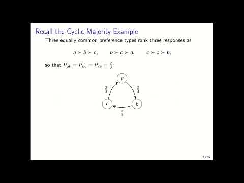
With three equally sized groups ranking A>B>C, B>C>A, and C>A>B, pairwise majorities form a rock-paper-scissors cycle.

14:00 Bradley-Terry Uses a Sigmoid of Reward Differences

The Bradley-Terry model assigns each completion a scalar reward rᵢ and predicts P(I beats J) = σ(rᵢ-rⱼ).
The logistic sigmoid approaches 1 for a large positive reward gap, 0 for a large negative gap, and 1/2 when rewards are equal.
Only reward differences affect predicted comparisons, so adding the same constant to every reward changes nothing.

17:00 Scalar Rewards Cannot Represent Comparison Cycles

A Bradley-Terry reward vector imposes a transitive ordering because σ is monotone in rᵢ-rⱼ.
The cyclic example requires rA>rB, rB>rC, and rC>rA, which no scalar reward vector can satisfy.
For a symmetric cycle, maximum likelihood assigns equal rewards and predicts 1/2 for each matchup, rather than fitting the population’s 2/3 win probabilities.

23:00 Reward Modeling Compresses Aggregate Preferences

A single reward model aggregates labelers with different preferences into one total ordering and necessarily loses information when preferences cycle.
Personalized reward models or multiple policies could preserve more user variation, though the data may not support a separate model for every person.
The Bradley-Terry model is a modeling choice, not a guarantee of a perfect population fit; its convenient optimization has consequences for what gets learned.

29:00 Constructing the Bradley-Terry Likelihood

For a comparison between I and J, encode the label as Y=1 when I is preferred and Y=0 otherwise.
If the reward difference is z, Bradley-Terry assigns probabilities σ(z) and σ(-z) to the two outcomes.
The likelihood for one label is σ(z)^Y σ(-z)^(1-Y), and maximizing likelihood is equivalent to maximizing log likelihood.

34:00 The Pairwise Logistic Negative Log-Likelihood

When the population win probability is p, the expected negative log-likelihood is -p log σ(z) -(1-p)log σ(-z).
Using the logistic form simplifies the objective to log(1+e^z)-pz.
For one pair, z can match any probability strictly between 0 and 1; the difficulty arises when reward differences must fit all pairs simultaneously.

39:00 Shared Reward Parameters Create a Misspecified Fit

With m completions, the model has m reward parameters but up to m² pairwise comparison probabilities to fit.
Each modeled difference must equal rᵢ-rⱼ, so independently chosen pairwise scores may not correspond to any consistent scalar reward vector.
Changing the loss or preprocessing can change the projection of cyclic population preferences onto a total ordering.

45:00 Borda Scores and the Reward-Modeling Theorem

The unnormalized Borda score of completion I is the sum of pᵢⱼ over every other completion J; the normalized score divides by m-1.
Borda ranks a response by its average chance of beating a randomly selected alternative in a randomly selected labeler’s comparison.
Roth states that any maximum-likelihood Bradley-Terry fit orders completions exactly as their population Borda scores do.

49:00 Deriving the Likelihood Gradient

Differentiating the pairwise loss with respect to reward difference z gives σ(z)-p.
This gradient is predicted win probability minus observed population win probability, the usual logistic-regression residual.
Because each reward appears in many comparisons, the derivative with respect to rᵢ must aggregate residuals across all opponents.

55:00 First-Order Conditions Match Borda Totals

At an unconstrained optimum, the gradient for every reward rᵢ is zero.
The resulting condition equates the sum of Bradley-Terry predicted win probabilities for I against all opponents with the sum of the population probabilities pᵢⱼ.
Adding the self-comparison term of 1/2 to both sums shows that fitted and population Borda totals match.

1:08:00 Monotone Rewards Recover the Borda Ordering

If fitted reward rᵢ exceeds rₖ, then I has a higher Bradley-Terry predicted win probability than K against every opponent J.
Summing over opponents makes I’s predicted Borda total strictly larger than K’s.
Since the fitted predicted totals equal population Borda totals, sorting rewards yields the Borda order, though reward values themselves are not Borda scores or utilities.

1:14:00 Reward-Only Policy Optimization Selects a Borda Winner

For a single prompt, a policy is a distribution over completions; maximizing predicted reward alone puts all probability on the highest-reward response.
Because reward order matches Borda order, reward-only optimization selects a Borda winner, or distributes mass among tied winners.
RLHF retains a pretrained base policy because pairwise preference labels do not supply the knowledge and capabilities learned during pretraining.

1:17:00 KL Regularization Constrains Policy Drift

The KL divergence from policy π to base policy π₀ is the expectation under π of log(π(I)/π₀(I)); it is nonnegative and zero only when the policies match.
The policy objective combines expected reward with a penalty weighted by τ for KL divergence from the pretrained policy.
This penalized objective corresponds to maximizing reward inside a KL-divergence budget: τ=0 allows unrestricted reward optimization, while very large τ keeps the base policy nearly unchanged.

1:21:00 Exponential Policy Tilting and the Copeland Alternative

The KL-regularized optimum is proportional to π₀(I)exp(rᵢ/τ), exponentially upweighting high-reward completions while retaining the base policy’s probabilities.
For two responses, the optimized log-odds shift from the base policy by (rᵢ-rⱼ)/τ, so numerical reward gaps matter when τ is positive.
Replacing comparison probabilities with binary wins before fitting can yield the Copeland ordering, which counts the fraction of opponents beaten by more than 1/2 instead of summing win probabilities.

Transcript excerpt

0:00 um pivot back from classical back to the machine learning and ask you okay like we've been thinking about um foundations of eliciting preferences but what does that actually imply for um what we're doing if we try learning a scalar reward model and then optimizing a a language model to high. So I just to like review a little bit this premise that we're going to train a reward model uh is that we're going to take a bunch of pair wise comparisons

0:48 that might exhibit all of the um difficulties that we've been talking about over the last few lectures for example and maybe no clean way to organize them to aggregate them into a total order. Um and yet we're going to try to like M to a scalar reward which will of course [cough] implicitly give some aggregation of them into a total um if we try to do that maybe one question we would immediately ask is what is the ordering that we're learning? We're not learning you know we're we're we're not learning something that is maximizing social welfare. We haven't even gathered the information necessary to like identify that problem. We're not

1:38 somehow respecting pairwise majority votes because we've seen that there's no total ordering that can do that. What are we doing? And what we're going to see is that the standard implementation is directly learning um a social choice rule we briefly saw before and has the name. It's learning the border. Um, and once you learn the reward model, you're not done. You you train the language model to um preferentially prefer highreward completions. And typically like you're going to have a base model that comes from pre-training and you don't want to entirely abandon everything you learn in the base model. So what you're

This is the start of the transcript. Save this video free for the whole transcript, searchable and time-coded.

Related notes

Summary, takeaways, and chapters were generated by AI from the video's transcript and may contain errors. The video belongs to its creator, Aaron Roth.