Linear Algebra for Engineers lecture 31: Orthogonal Projections and Orthonormal Sets
Overview
Alex Townsend develops orthogonal projection as the geometric shadow of a vector onto a line, then uses it to calculate nearest-point distances. He shows how orthonormal bases simplify coordinates and projections, and how a square matrix with orthonormal columns satisfies UᵀU = I and U⁻¹ = Uᵀ, motivating Gram–Schmidt and QR factorization.
Key takeaways
- For a nonzero vector u spanning a line, the orthogonal projection of b is ((uᵀb)/(uᵀu))u; replacing u by any nonzero scalar multiple does not change the projected point.
- The shortest distance from b to a line is the length of the residual after projection: ‖b − projₗ(b)‖.
- An orthonormal basis makes the coordinates of b especially simple: cᵢ = uᵢᵀb, because every basis vector has squared length 1.
- For a matrix U with orthonormal columns, UᵀU = I; if U is square, this also gives U⁻¹ = Uᵀ and makes solving Ux = b a transpose multiplication.
- Orthogonal columns alone do not make U⁻¹ equal Uᵀ: their squared lengths remain on the diagonal of UᵀU unless each column is normalized.
Chapters
- Vectors are orthogonal when their dot product xᵀy is zero; the zero vector is orthogonal to every vector.
- For an orthogonal basis, each coordinate is cᵢ = (uᵢᵀb)/(uᵢᵀuᵢ), avoiding elimination and augmented matrices.
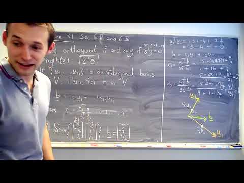
- Alex Townsend checks that (1, −4, 2) and (3, 1, 1/2) are orthogonal because their dot product is zero.
- Townsend decomposes a vector B into perpendicular components c₁u₁ and c₂u₂.
- Each component is the orthogonal shadow of B onto the line spanned by its basis vector.
- For the example basis (1, −4, 2) and (3, 1, 1/2), the coordinates are 2 and 1.
- The line y = x is spanned by u = (1, 1), and the vector being projected is b = (1, 0).
- Using projₗ(b) = (uᵀb)/(uᵀu)u gives 1/2(1, 1).
- Rescaling the spanning vector to (2, 2) leaves the projection unchanged because the common scale factors cancel.
- For b = (7, 6) and the line spanned by u = (4, 2), the projection coefficient is (uᵀb)/(uᵀu) = 40/20 = 2.
- The nearest point on the line is b̂ = 2u = (8, 4).
- The shortest distance is ‖b − b̂‖ = ‖(−1, 2)‖ = √5; the perpendicular segment gives the minimum.
- An orthonormal set has mutually perpendicular vectors of length 1, so uᵢᵀuⱼ = 0 for i ≠ j and uᵢᵀuᵢ = 1.
- If an orthonormal set spans V, it is automatically a basis because its vectors are nonzero and orthogonal.
- For b in V, the coordinate formula reduces to cᵢ = uᵢᵀb, with no division by a squared length.
- Divide (1, −4, 2), whose length is √21, by √21 to make it a unit vector.
- The vector (3, 1, 1/2) has length √41/2, so its normalized form is (6, 2, 1)/√41.
- Scaling each nonzero vector preserves the 90-degree angle, producing an orthonormal basis from the original orthogonal one.
- Townsend forms a matrix U by placing basis vectors in its columns.
- Each entry of UᵀU is a dot product between two columns: off-diagonal entries are zero and diagonal entries are one.
- For an m-by-n matrix U with orthonormal columns, UᵀU = Iₙ, including when U is rectangular.
- When U is square and its columns are orthonormal, UᵀU = I implies U⁻¹ = Uᵀ.
- Solving Ux = b then requires only x = Uᵀb, rather than Gaussian elimination.
- Townsend previews the Gram–Schmidt algorithm for constructing orthonormal bases and QR factorization as a related matrix factorization.
- The term orthogonal matrix refers to a square matrix with orthonormal columns, not merely perpendicular columns.
- With orthogonal but non-unit columns, UᵀU has squared column lengths on its diagonal rather than ones, so U⁻¹ is not simply Uᵀ.
- Townsend notes that orthogonal columns can be normalized, which is why applications commonly use orthonormal columns.
- Townsend begins a question about the eigenvalues and eigenvectors of an orthogonal matrix.
- The class considers whether eigenvalues might be 1, but the lecture ends before completing the discussion.
Transcript excerpt
0:00 is in lecture 31 which is section 6.2 and a bit of section 6.3 of the textbook. So we're we're just learning right now uh about orthogonality and as the lectures go on we're going to start using orthogonality and I showed you last time how one aspect of orthogonality was super useful when you want to work when you're working in a basis that's an orthogonal set then uh that can be really convenient. So we say two vectors are orthogonal if their dot product is zero. This is the linear algebra uh notation for dotproduct. It means x is a column vector. Y is a column vector. So here is a one by n matrix or vector, right? And here is that's xrpose and y is like an n
0:52 by one. So the output is a one by one matrix matrix multiplication. You get a number out of it. If that number is zero, they're orthogonal. This includes the zero vector. So the zero vector is the only vector that's orthogonal to itself. The zero vector is orthogonal to every vector. We know that we can calculate the length of a vector through this formula which is kind of another like sum up the anyway you square every entry sum them up and then you take the square root. Um if you're given an orthogonal basis that's really [clears throat] nice um because if you want to work in that basis the first thing you need to do is to work out the coordinates right the the the C1 CN
1:40 so that you can write B as a linear combination of your bases and that's really easy when you have orthogonality orthogonal vectors because we worked out last time this little neat formula which is a number divided by a
This is the start of the transcript. Save this video free for the whole transcript, searchable and time-coded.
In this course
Related notes
Summary, takeaways, and chapters were generated by AI from the video's transcript and may contain errors. The video belongs to its creator, Alex Townsend.