Linear Algebra for Engineers lecture 29: Oscillations from Complex Eigenvalues
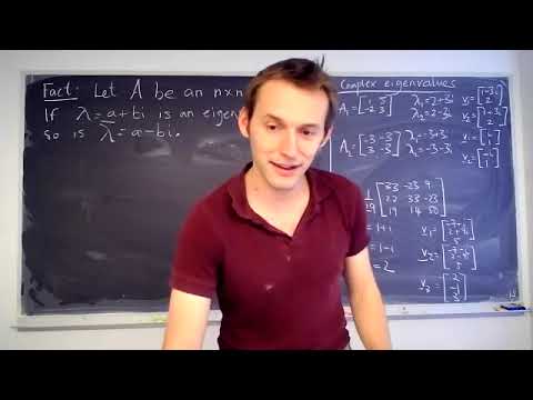
Overview
Alex Townsend explains how complex eigenvalues in real linear systems produce real oscillations: conjugate eigenvalue and eigenvector pairs combine so their imaginary parts cancel. He applies the method to a spring with mass and spring constant both 1, converting its second-order equation into a 2×2 system and recovering sine and cosine motion from eigenvalues ±i.
Key takeaways
- For a real matrix A, every nonreal eigenvalue λ = a + bi is accompanied by λ̄ = a − bi, and an eigenvector v is accompanied by its conjugate v̄.
- Complex exponentials e^(it) and e^(−it) combine into real cosine and sine terms, explaining why complex eigenvalues model real oscillations.
- The spring equation m x″ + kx = 0 becomes the first-order system x′ = v, v′ = −x when m = k = 1; with x(0) = 0 and v(0) = 1, its solution is x(t) = sin(t), v(t) = cos(t).
- Real eigenvalues describe exponential modes: positive eigenvalues grow, negative eigenvalues decay, and a zero eigenvalue yields a constant mode.
- A real 2×2 or 3×3 matrix with a nonreal eigenvalue must be diagonalizable because its conjugate pair, together with any remaining real eigenvalue, gives distinct eigenvalues.
- Every odd-dimensional real matrix has at least one real eigenvalue because its nonreal eigenvalues occur in pairs.
Chapters
- The lecture revisits systems of the form y′ = Ay and the solution method based on diagonalizing A.
- In eigenvector coordinates, each component evolves through an exponential e^(λt).
- Real positive eigenvalues produce exponential growth, negative ones produce decay, and a zero eigenvalue produces a constant component.
- For z = a + bi, the complex conjugate is z̄ = a − bi, formed by changing the sign of the imaginary part.
- Townsend compares eigenvalues of several real matrices and observes that nonreal eigenvalues occur in conjugate pairs.
- The same pairing appears in the corresponding eigenvectors, allowing complex calculations to yield real-valued results.
- The characteristic polynomial of a real matrix has real coefficients, so its nonreal roots occur in complex-conjugate pairs.
- If Av = λv for a real matrix A, conjugating both sides gives A v̄ = λ̄ v̄.
- Thus, an eigenvector v for λ has conjugate eigenvector v̄ for λ̄.
- Townsend models a mass m on a spring with spring constant k and displacement x(t) from the spring’s anchor.
- Newton’s law and Hooke’s law give m x″(t) = −k x(t), or m x″(t) + kx(t) = 0.
- The example uses m = 1 and k = 1, with initial displacement x(0) = 0 and initial velocity x′(0) = 1.
- Defining velocity as v(t) = x′(t) replaces the second-order equation with two first-order equations.
- For m = k = 1, the system is x′ = v and v′ = −x.
- In vector form, [x′, v′]ᵀ = [[0, 1], [−1, 0]][x, v]ᵀ, making the problem one of linear algebra.
- The matrix [[0, 1], [−1, 0]] has characteristic equation λ² + 1 = 0.
- Its eigenvalues are +i and −i, a complex-conjugate pair.
- One eigenvector for +i is [1, i]ᵀ, and its conjugate [1, −i]ᵀ corresponds to −i.
- Townsend uses the solution formula y(t) = P e^(Dt) P⁻¹ y(0), with columns of P given by the two eigenvectors.
- Here D has diagonal entries i and −i, while the initial state is [x(0), v(0)]ᵀ = [0, 1]ᵀ.
- At t = 0, the exponential matrix becomes the identity, so the formula reproduces the specified initial conditions.
- The terms e^(it) and e^(−it) combine using Euler’s formula to produce real sine and cosine functions.
- For the stated initial conditions, the displacement is x(t) = sin(t) and the velocity is v(t) = cos(t).
- The conjugate eigenvalue contributions cancel imaginary parts, leaving real-valued periodic motion.
- A real 2×2 matrix with a nonreal eigenvalue also has its distinct conjugate, so it has two distinct eigenvalues and is diagonalizable.
- A real 3×3 matrix with a nonreal eigenvalue has a conjugate pair plus one real eigenvalue; all three are distinct, so it is diagonalizable.
- For real 4×4 and larger matrices, repeated eigenvalues can occur, so the presence of a complex pair alone does not guarantee diagonalizability.
- Nonreal eigenvalues of a real matrix pair up with their conjugates, accounting for an even number of eigenvalues when counted with multiplicity.
- An odd-dimensional real matrix, such as a 15×15 or 37×37 matrix, must therefore have at least one real eigenvalue.
- For an even-dimensional real matrix, this pairing argument alone does not guarantee any real eigenvalues.
Transcript excerpt
0:00 I heard that something like that exists. Okay. Um the the uh the se the okay the pain and suffering I should just say it one last time uh is in 5.57 of the textbook today. So this is complex values differential equations. So my goal today is to show you how complex I values have real world consequences. And the the main message is complex values give you oscillations. Now I'll show you what that means. They give you oscillating behaviors. So okay so last time we were looking at solving this um these kind of equations. So there I had a I had in one example I had n equals two. One of these functions
0:48 meant the amount of steroid in the muscle. One of these functions was about the amount of steroid in the bloodstream. And we were trying to understand how they evolve with time. If I inject some steroid in the muscle, how does it change the amount of steroid in the bloodstream over time? And we we in that one case we had a equation like this which tells us that the rates of change of the variables of interest the functions of interest that's what this is the bar means uh so this means the rate of change here if I did that I would have to come here and do that right they all get derivatives individually then uh they're connected by their own values the rates of change depend on the
1:36 values of all the other things like if I had more steroid in the muscle that would seep into the blood so it would increase the rate of change of the function about steroid in the blood and so they're all connected with this matrix A which all it does is a linear
This is the start of the transcript. Save this video free for the whole transcript, searchable and time-coded.
In this course
Related notes
Summary, takeaways, and chapters were generated by AI from the video's transcript and may contain errors. The video belongs to its creator, Alex Townsend.