L4 Pauli Matrices and Spin Operator
 Watch on YouTube →
Overview
Hiu-Yung Wong connects the linear-algebra foundations of quantum states to the Pauli matrices, deriving the σx eigenstates and reviewing how σx, σy, and σz act on a two-dimensional spin space. He then explains their algebraic identities and physical interpretation, culminating in the arbitrary-direction spin operator n·σ and its explicit 2×2 matrix.
Key takeaways
- The eigenstates of σx are |+⟩ = (|0⟩ + |1⟩)/√2 and |−⟩ = (|0⟩ − |1⟩)/√2, with eigenvalues +1 and −1.
- Each Pauli matrix squares to the identity, while distinct Pauli matrices anticommute: {σi, σj} = 2δijI.
- The identity and three Pauli matrices form a basis for every 2×2 Hermitian matrix using four real coefficients.
- Spin-up and spin-down are defined relative to a chosen magnetic-field axis; changing the field from z to x changes the measurement eigenbasis.
- For direction n = (nx, ny, nz), the spin operator n·σ is [[nz, nx − i ny], [nx + i ny, −nz]].
Chapters
- A two-state system is represented by a vector that is a scalar linear combination of |0⟩ and |1⟩.
- The |+⟩ and |−⟩ basis is an alternative representation of the same state, found by substituting their expressions in the computational basis.
- A ket has a corresponding bra; scalar coefficients are complex-conjugated when converting a ket combination into its bra.
- Swapping the order of an inner product gives its complex conjugate, so the two orders are equal when the result is real.
- A normalized state satisfies ⟨a|a⟩ = 1, which means its vector has unit length.
- An operator is represented by a matrix that acts on a state vector; an eigenvector is mapped to a scalar multiple of itself.
- In the computational basis, σz is the diagonal matrix with entries 1 and −1, so |0⟩ and |1⟩ are its eigenvectors.
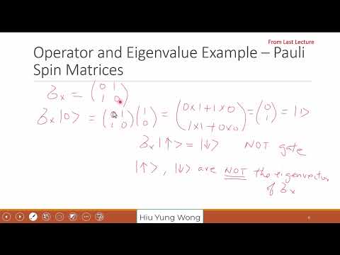
- The Pauli matrix σx = [[0, 1], [1, 0]] maps |0⟩ to |1⟩ and |1⟩ to |0⟩.
- Because σx changes the computational basis states rather than scaling them, |0⟩ and |1⟩ are not σx eigenvectors.
- Write a candidate eigenvector as a|0⟩ + b|1⟩ and impose σx|v⟩ = λ|v⟩.
- Matching components gives b = λa and a = λb, which requires λ² = 1.
- The two eigenvalues are +1 and −1, with coefficient relationships b = a and b = −a, respectively.
- Normalizing the coefficient pairs (a, a) and (a, −a) gives |+⟩ = (|0⟩ + |1⟩)/√2 and |−⟩ = (|0⟩ − |1⟩)/√2.
- An eigenvector can be multiplied by any nonzero scalar and remain an eigenvector; after normalization, an overall phase still gives an equivalent quantum state.
- The σx eigenbasis is therefore the plus/minus basis, distinct from the computational basis.
- The Pauli matrices are σx = [[0, 1], [1, 0]], σy = [[0, −i], [i, 0]], and σz = [[1, 0], [0, −1]].
- They may also be indexed as σ1, σ2, and σ3; σ0 denotes the 2×2 identity matrix.
- The matrices act on a two-dimensional state space, while their x, y, and z labels connect to spatial measurement directions.
- Direct matrix multiplication shows σx² = I, and the same identity holds for σy² and σz².
- This makes repeated identical Pauli operations simplify: an even number of σx operations reduces to I.
- The identity matrix leaves a state unchanged, avoiding unnecessary repeated matrix multiplications.
- The anticommutator is defined as {A, B} = AB + BA, while the commutator is [A, B] = AB − BA.
- The Pauli matrices satisfy {σi, σj} = 2δijI: equal indices yield 2I, and distinct indices yield the zero matrix.
- For example, σxσy + σyσx = 0; matrix multiplication order cannot generally be swapped.
- The matrices I, σx, σy, and σz form a four-element basis for the real vector space of 2×2 Hermitian matrices.
- Any 2×2 Hermitian matrix can be expressed as αI + βσx + γσy + δσz, with real coefficients α, β, γ, and δ.
- Wong notes that matrix inner products can be defined using the trace, a tool relevant to decomposing operators in quantum circuits.
- Without an external magnetic field, spin-up and spin-down states have the same energy in the example discussed.
- A field along z lifts the degeneracy, allowing the two states to be distinguished by their different energy levels.
- Spin labels refer to measurement relative to a chosen field direction; the precise energy ordering depends on the particle and its coupling.
- The labels up and down are relative to the direction of the magnetic field, not an absolute direction in space.
- A field along x uses σx rather than σz, so the corresponding spin eigenstates differ from |0⟩ and |1⟩.
- The same two-level spin structure applies along x, y, or z, consistent with spatial isotropy.
- An arbitrary real-space direction is written n = nx x̂ + ny ŷ + nz ẑ, where nx, ny, and nz are real components.
- The Pauli-vector notation combines the three matrices as σ = σx x̂ + σy ŷ + σz ẑ.
- Taking the dot product n·σ selects the Pauli operator associated with the chosen direction.
- The Pauli vector can be displayed as a column whose entries are the matrices σx, σy, and σz, rather than ordinary scalar components.
- This construction combines real-space basis directions with matrix-valued coefficients.
- The notation prepares the calculation of a spin operator for a field pointing in any direction.
- Taking n·σ gives nxσx + nyσy + nzσz, a single 2×2 operator for the selected direction.
- Substituting the Pauli matrices yields [[nz, nx − i ny], [nx + i ny, −nz]].
- This matrix is the spin operator associated with direction n; its eigenstates describe spin aligned or anti-aligned with that direction.
Transcript excerpt
0:07 reading the book after this class or yeah or this week you should be have uh read chapter 1 to six is a complimentary so what did we learn from the last lecture I want to remind you some of the important concepts right so first of all in the previous lectures we already talked about cubit oh not cubit a state a few the The state of a a physical system is represented by a vector. And here we have a special case. How what is the dimension of this system? Two, right? Because it has two basis states zero and one. And we express this as a general linear combination of zero and one. So what are A and B? Are they vector matrix or lumbers or what?
0:56 Scalers. Yeah, lumbers, right? And they can be compressed right and then we say okay uh we represent them in the zero and one basis if it is given as zero equal to this combination of another basis. So we have zero and one basis. We also have plus minus bases. Again there's nothing special. It's just a name, right? Just like the eight analogy. Uh 24x equal to two one two dozen eggs, right? So dozen one dozen egg and one x are two different bases, right? But they are equivalent. So same I can express this vector as a linear combination of plus and minus, right? All I need to do just do the substitution of zero equal
1:43 to this and one equal to this. This a different this equation. Okay. Is that okay this concept? Any questions? This is a two dimension. Uh then if you go to n dimension everything is the same. We also talk about the bra cat uh notation and their duality right their
This is the start of the transcript. Save this video free for the whole transcript, searchable and time-coded.
Related notes
Summary, takeaways, and chapters were generated by AI from the video's transcript and may contain errors. The video belongs to its creator, Quantum Computing, TCAD, Semicond by Hiu-Yung Wong.