L7 Projection Operator, Measurement, Hilbert Space and Tensor Product

Overview

Hiu-Yung Wong develops projection operators as outer products and connects them to measurement probabilities through the Born rule, including a three-state example where outcomes 1 or 2 have probability 2/3. He then defines Hilbert spaces and shows how tensor products combine subsystem states and operators, producing an n-dimensional-by-m-dimensional space of dimension nm and an n-qubit space of dimension 2^n.

Key takeaways

For a normalized target vector |v⟩, the projector |v⟩⟨v| extracts the component of |α⟩ along |v⟩, returning ⟨v|α⟩|v⟩.
Measurement in an orthonormal basis gives outcome j with probability ⟨α|Pⱼ|α⟩ = |⟨j|α⟩|² = |αⱼ|²; the projector computes a probability, not a deterministic measurement result.
For the normalized three-state example with amplitudes 1/√3, −i/√3, and 1/√3, each basis outcome has probability 1/3, so the combined probability of outcomes 1 or 2 is 2/3.
A Hermitian observable such as Pauli Z for spin along z has real eigenvalues that represent possible outcomes; projectors onto its eigenstates determine their Born-rule probabilities.
Tensor products multiply dimensions: combining n- and m-dimensional spaces gives dimension nm, while n qubits span a 2ⁿ-dimensional space.
Tensor products of operators combine subsystem actions without ordinary matrix multiplication; for two single-qubit 2 × 2 operators, the joint operator is a 4 × 4 matrix.

Chapters

0:00 Course Notice and Linear-Algebra Toolkit

Poster assignment 1 is due September 23; during next week's travel, Hiu-Yung Wong plans to post recorded lessons and offer office hours or Zoom meetings.
The lecture extends the quantum-computing linear-algebra toolkit, moving from unitary and Hermitian matrices to projection operators.

0:33 Projection Operators as Outer Products

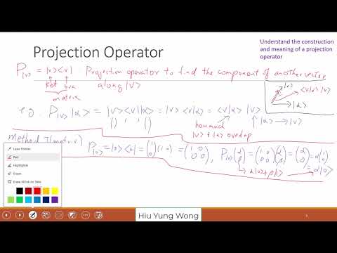
The projector onto a normalized vector |v⟩ is |v⟩⟨v|, an outer product that produces a matrix.
A projector selects the component of another vector along |v⟩; identifying bras, kets, scalars, and matrices helps prevent notation errors.

3:00 Applying a Projector to Extract a Vector Component

Applying |v⟩⟨v| to |α⟩ gives |v⟩⟨v|α⟩ = ⟨v|α⟩|v⟩.
The inner product ⟨v|α⟩ supplies the component's scalar size, while the resulting vector points along |v⟩.
For unit vectors in a familiar 2D picture, the overlap corresponds to the component along |v⟩, analogous to a cosine factor.

9:00 Computing the Qubit Projector P₀

For |0⟩ = (1, 0)ᵀ, the projector P₀ = |0⟩⟨0| is the matrix [[1, 0], [0, 0]].
Applying P₀ to α|0⟩ + β|1⟩ returns α|0⟩, removing the orthogonal |1⟩ component.
P₀ is not unitary, so it is not a quantum gate; it can instead be used to calculate a measurement probability.

13:00 Born-Rule Probability from a Projection Operator

For a normalized state |α⟩ and basis outcome |j⟩, the probability is ⟨α|Pⱼ|α⟩, where Pⱼ = |j⟩⟨j|.
Expanding the expression gives |⟨j|α⟩|² = |αⱼ|², matching the coefficient-squared rule for a measurement in that basis.
The projector formula generalizes the familiar basis-measurement calculation and prepares for more general measurement descriptions.

16:00 Measurement Outcomes in an n-Dimensional Basis

A state |α⟩ = Σⱼ₌₀ⁿ⁻¹ αⱼ|j⟩ has n basis states, from |0⟩ through |n−1⟩.
Measuring in that basis yields one of its basis states; the chance of outcome j is |αⱼ|².
The computational basis is one measurement basis; changing the basis changes which components the measurement tests.

21:00 Deriving the Probability Formula with Bras and Kets

Substituting Pⱼ = |j⟩⟨j| into ⟨α|Pⱼ|α⟩ yields ⟨α|j⟩⟨j|α⟩.
The two inner products are complex conjugates, so their product is |⟨j|α⟩|².
Expanding |α⟩ in an orthonormal basis leaves only the jth term in ⟨j|α⟩, producing |αⱼ|².

27:00 Three-State Example: Probability of Outcomes 1 or 2

For |s⟩ = (1/√3)|0⟩ − (i/√3)|1⟩ + (1/√3)|2⟩, the three coefficient magnitudes squared are each 1/3.
The state is normalized because the three outcome probabilities sum to 1.
The probability of outcome 1 or outcome 2 is P(1) + P(2) = 2/3; this is not the probability of projecting onto the superposition |1⟩ + |2⟩.

33:00 Complex-Conjugate Amplitudes in Projector Calculations

When forming ⟨s| from |s⟩, the coefficient −i/√3 becomes +i/√3 through complex conjugation.
In ⟨s|P₁|s⟩, orthogonality eliminates terms involving |0⟩ and |2⟩, leaving the outcome-1 probability of 1/3.
Careful conjugation matters: multiplying the surviving amplitude by its conjugate produces a real, nonnegative probability.

40:00 Observables, Hermitian Matrices, and Measurement Outcomes

A quantum observable is represented by a Hermitian operator; the example of spin measured along z uses the Pauli Z matrix.
The possible outcomes of that spin measurement are the operator's eigenvalues, +1 and −1.
The probability of an eigenstate outcome is calculated with its projector, Pᵢ = |λᵢ⟩⟨λᵢ|, using the Born rule.

44:00 Hilbert Space: Inner Products and Completeness

A Hilbert space is a complete linear space equipped with a defined inner product.
The inner product must be positive for a vector with itself, conjugate-symmetric when its arguments are swapped, and compatible with addition.
Every finite-dimensional inner-product space is complete; completeness becomes a more substantial issue for infinite-dimensional spaces.

52:00 Combining Two Qubit Systems with Tensor Products

A two-qubit joint state is formed by tensoring the states of the two subsystems, such as (α|0₁⟩ + β|1₁⟩) ⊗ (γ|0₂⟩ + δ|1₂⟩).
Distributing the tensor product gives four terms with coefficients αγ, αδ, βγ, and βδ.
Subsystem labels distinguish which qubit each basis state belongs to; the order must remain consistent when writing the joint state.

59:00 Two-Qubit Basis Labels and Decimal Indexing

The two-qubit basis states |00⟩, |01⟩, |10⟩, and |11⟩ can be abbreviated by decimal indices 0 through 3.
Those decimal labels encode binary bit strings: for example, index 2 represents |10⟩ and index 3 represents |11⟩.
The coefficient vector for the general product state is (αγ, αδ, βγ, βδ)ᵀ in the stated basis order.

1:05:00 Tensor-Product Dimensions for Multiple Qubits

A single qubit has two basis states and a two-dimensional complex state space; two qubits have four basis states and dimension 4.
Three qubits have 2 × 2 × 2 = 8 basis states, and n qubits have 2ⁿ basis states indexed from 0 to 2ⁿ−1.
Tensoring spaces of dimensions n and m produces a space of dimension nm, not n + m.

1:11:00 Expanding Tensor Products of State Vectors

For vectors v = Σᵢ vᵢ|eᵢ⟩ and w = Σⱼ wⱼ|fⱼ⟩, distribute the tensor product to obtain Σᵢⱼ vᵢwⱼ(|eᵢ⟩ ⊗ |fⱼ⟩).
The resulting vector has nm entries because every one of the n components of v pairs with every one of the m components of w.
In column-vector form, the entries appear as products such as v₀w₀ through v₀wₘ₋₁, followed by the corresponding products for each later v component.

1:14:30 Building Joint Operators with Matrix Tensor Products

Operations acting on two subsystems combine as U₁ ⊗ U₂, paralleling the tensor-product construction for state vectors.
For 2 × 2 matrices U₁ = [[A, B], [C, D]] and U₂ = [[E, F], [G, H]], their tensor product is a 4 × 4 block matrix.
Each entry of U₁ multiplies the entire matrix U₂, producing blocks AU₂, BU₂, CU₂, and DU₂ rather than an ordinary matrix product.

Summary, takeaways, and chapters were generated by AI from the video's transcript and may contain errors. The video belongs to its creator, Quantum Computing, TCAD, Semicond by Hiu-Yung Wong.