ISE 754 (Fall 2026) 5.3 Vehicle Routing
Overview
Michael G. Kay explains how vehicle routing extends earlier routing methods by adding constraints such as vehicle capacity, maximum route cost, time windows, and hours of service. The central technique sets a route's cost to infinity whenever a route-level constraint is violated, allowing methods such as Clarke-Wright savings and minimum insertion to reject infeasible routes; the lecture also distinguishes routes from vehicles and discusses pickup-delivery loads, vehicle assignment, and tactical estimates.
Key takeaways
- Assigning infinite cost to a route that violates capacity or another route-level rule lets standard savings and insertion heuristics exclude it without redesigning the entire routing procedure.
- A solution requiring two routes may need only one vehicle if it can complete one route, return to the depot to reload, and perform the next route in sequence.
- For pickup-delivery routing, capacity depends on the largest quantity onboard at any point, so every distinct load mix along a route must be checked.
- The Savannah-to-Gainesville shipment remains separate from shipments 1 and 2 in the example because combining it would exceed vehicle capacity during the final route segment.
- Minimizing the number of vehicles is a distinct fleet-planning objective from minimizing total route cost, and the lecture's Model 3 states the objective but does not solve it.
- Tactical TSP distance estimates can help plan approximate fleet size, route count, capacity needs, and delivery time without constructing exact routes.
Chapters
- Equation 1 assigns a route its ordinary distance, travel-time, or transport-dollar cost when total shipment load is within vehicle capacity, and infinity when capacity is exceeded.
- Clarke-Wright savings and minimum insertion then avoid infeasible routes because infinite cost makes the alternative unattractive or its savings negative infinity.
- Capacity, maximum route cost, time windows, and hours-of-service rules can be handled when each constraint applies to one route; limits on total or maximum route counts involve multiple routes and are outside the covered procedures.
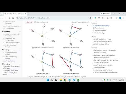
- With a capacity of 15 units, the example produces two routes with loads of 15 each; two routes do not necessarily mean two vehicles, since one vehicle might reload at the depot between trips.
- Mixed pickups and deliveries require checking the maximum onboard load during each segment, not simply adding every shipment assigned to a route.
- A route that picks up shipments 1, 2, and 3 before delivering them has one load mix; delivering shipment 1 before picking up 3 creates separate mixes of shipments 1 and 2, then 2 and 3.
- In the southeastern United States example, shipments 1 and 2 can be consolidated, but shipment 3 from Savannah to Gainesville must remain independent because including it would exceed capacity near the route's end.
- Absolute time windows require a vehicle to reach a location within its specified interval; arriving outside the interval makes the route infeasible.
- Model 3 proposes a two-stage objective: first minimize the number of vehicles, then minimize total route cost among solutions using the fewest vehicles; the lecture does not provide a solving procedure for this model.
- The routing procedures covered focus on total route cost, while assigning vehicles to routes and minimizing fleet size require additional methods.
- A TSP distance-estimation formula can support tactical planning, including estimates of route count, vehicle capacity, delivery time, and vehicles to rent for an upcoming week.
Transcript excerpt
0:00 We will be covering the vehicle routing problem. It is similar to the previous routing problems that we considered before. The only difference is that now the vehicles have different types of limitations or capacity constraints. So as a result of that, to be able to solve a problem, we can end up having to require multiple routes. The key to what is done to enforce these types of constraints is equation one of the lecture. And here what it basically is saying is that the cost of a particular route R is
0:48 whatever the cost would be, which would typically be either distance or travel time, or it could actually be the dollars associated with transporting the product. And that's the cost if the sum of the load, the shipments that are in the load being transported is less than some capacity of the vehicle. In cases where it then exceeds it, we just set the cost equal to infinity. And the reason it works is that things like the minimum insertion procedure or the savings procedure considered in the previous lecture, when we have a cost of infinity, it makes it such that that savings is going to be negative infinity, so
1:34 there's no positive savings. So it would never make sense to actually insert it. Or in terms of minimum cost, having it equal to infinity is never going to be the optimal way to solve things. So as long we basically then just have to encode our capacity constraints by some procedure that when we violate the constraints, we just set the cost of the route to infinity. And then at that point, everything that we've already about in routing carries through to the vehicle routing problem. That is really in essence how we're going to approach these problems.
This is the start of the transcript. Save this video free for the whole transcript, searchable and time-coded.
In this course
Related notes
Summary, takeaways, and chapters were generated by AI from the video's transcript and may contain errors. The video belongs to its creator, Michael G. Kay.