Intro to Statistics at IU Indy - One-Sample Tests Lecture 1
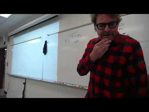
Overview
Andy Baker introduces one-sample hypothesis tests for IU Indy students, starting with how to express claims as null and alternative hypotheses and distinguish two-tailed tests from directional one-tailed tests. He connects a 95% confidence level to alpha = 0.05, explains rejection versus failure to reject, and outlines sample assumptions, choosing Z or t procedures, test statistics, and the two-tailed Z critical values of ±1.96.
Key takeaways
- A null hypothesis represents the stated population claim and must include equality; for a claim of a 20% first-generation student proportion, write H₀: p = 0.20.
- The alternative hypothesis determines the tail: use p or μ not equal to the claimed value for a two-tailed test, greater than for a right-tailed test, and less than for a left-tailed test.
- At a 95% confidence level, α = 0.05; a two-tailed test divides that error area into 0.025 per tail and uses Z critical values of approximately −1.96 and +1.96.
- Choose a Z test when population σ is known or the sample is large; choose a t test when σ is unknown or the sample is small, using n − 1 degrees of freedom.
- Before testing, check that sampling is random and observations are independent; with a small-sample t test, also check that the original data are approximately normally distributed.
- Failing to reject H₀ does not establish that a claim is true; it means the sample evidence was not sufficiently extreme to reject it.
Chapters
- Andy Baker reminds students that Quiz 8 is next class and that its Canvas sample questions will resemble the quiz with different scenarios and data.
- Labs 1 through 6 have been graded; submitted work generally earns strong scores, while missing labs are costing students points.
- Baker recommends completing labs in smaller sessions instead of waiting until the Sunday 10:55 or 11:55 p.m. deadline.
- Quiz 7 results show improvement, including strong performance on the final question about the most recent course material.
- Baker offers to explain quiz deductions in person, during Thursday office hours, or by email with a photo of the work.
- The course project proposal is due Sunday, November 1; students should submit agreed project plans in Canvas even after discussing them with Baker.
- Project ideas should connect to course statistics and be interesting to the student, rather than aiming at publication or a large research study.
- A prior 10-minute online lecture contrasts snowball and convenience sampling with the truly random samples assumed in statistical tests.
- Hypothesis testing uses data to evaluate claims instead of relying on unsupported theories or a few agreeing opinions.
- Baker frames the coming lectures as a progression from one-sample tests to comparisons between two samples, such as before-and-after observations or separate groups.
- The null hypothesis, written H₀, represents the stated claim or status quo; the alternative, Hₐ, expresses a competing possibility.
- For a campus flyer claiming one in five IU Indy students is first-generation, the hypotheses are H₀: p = 0.20 and Hₐ: p ≠ 0.20.
- For a claim that the mean weekly grocery bill is $40, use the population parameter μ: H₀: μ = 40 and Hₐ: μ ≠ 40.
- Use p for a population proportion and μ for a population mean, rather than sample statistics such as p-hat or x-bar in the hypotheses.
- For a claim that 20% of IU Indy students bike to campus, the parameter is p; whether the test is directional depends on the research question.
- If the claim is that the mean is two campus library visits per week and the suspected value is higher, write H₀: μ ≤ 2 and Hₐ: μ > 2.
- For a 30% campus meal-plan claim, a suspected higher proportion gives H₀: p ≤ 0.30 and Hₐ: p > 0.30; a suspected lower proportion reverses the inequalities.
- Baker emphasizes that the null hypothesis always includes equality.
- A one-sample test compares data from one collected sample with a claim about a population parameter.
- The first step is to state the research question and write H₀ and Hₐ, identifying what the study is trying to investigate.
- A sample that is close to the claimed value may fail to provide evidence against the claim, while an extreme result may prompt rejection.
- A two-tailed test asks whether a value is different in either direction, as in asking whether IU Indy students' GPA differs from the national average.
- A right-tailed test is appropriate when the research claim predicts a higher value, such as expecting improved student retention.
- A left-tailed test predicts a lower value, such as asking whether Indiana manufacturing wages are below the national average.
- The alternative hypothesis signals the direction: not equal means two-tailed, greater than means right-tailed, and less than means left-tailed.
- Baker uses alpha = 1 − confidence level, so a 95% confidence level gives α = 0.05.
- In a one-tailed test, the full 0.05 rejection probability is placed in one tail; in a two-tailed test, it is split into 0.025 per tail.
- An alpha of 0.01 would correspond to a 99% confidence level, although the course mainly uses 0.05.
- The rejection regions are the tail areas associated with alpha; a two-tailed test at α = 0.05 has 0.025 in each tail.
- A result in a rejection region leads to rejecting H₀ because the sample is unusually far from the claimed value.
- A result in the central, 95% fail-to-reject region means the evidence is insufficient to reject H₀.
- Baker cautions that failing to reject does not prove the claim is true; it means the sample has not shown it to be false.
- The 20% student-biking claim becomes a two-tailed test if the research question asks whether the proportion is different, without predicting higher or lower.
- The library-visit claim is also two-tailed when the suspected mean is simply different from two visits per week.
- Baker notes that academic journals often prefer two-tailed tests because a one-tailed test can miss an effect in the unpredicted direction.
- Use a Z test when the population standard deviation σ is known or when the sample is large, described here as roughly more than 30 to 40 observations.
- Use a t test when σ is unknown, which Baker says is common, or when the sample is small.
- Sigma refers to the population standard deviation, while s refers to the sample standard deviation.
- A t test uses degrees of freedom equal to n − 1; for example, n = 36 gives 35 degrees of freedom.
- The sample should be truly random, not just a survey distributed to people nearby or otherwise selected by convenience.
- Observations should be independent; commuting times may be dependent when respondents carpool, and two people completing a survey together can influence each other's answers.
- For a t test with a small sample, especially around 10 observations or fewer, the original data should be roughly normally distributed rather than strongly bimodal.
- These three conditions are assumptions to check when conducting research with collected data.
- For a mean with a Z test, calculate z = (x-bar − μ₀) / (σ / √n), comparing the sample mean with the claimed population mean.
- The t statistic follows the same general comparison but uses the sample standard deviation s when population σ is unknown.
- For a proportion, use a Z statistic rather than a t test; the standard error is based on the claimed proportion p₀.
- In Baker's example, if the first-generation claim is p₀ = 0.20 and a sample of 100 finds 13%, p-hat is 0.13 and the comparison is against 0.20.
- For a two-tailed Z test with α = 0.05, the critical values are −1.96 and +1.96, leaving 0.025 in each rejection tail.
- A test statistic between −1.96 and +1.96 falls in the fail-to-reject region; a statistic beyond either boundary falls in a rejection region.
- Baker distinguishes an extreme result from one close to zero: extreme results support rejecting the claim, while results close to the claimed value do not.
- The lecture ends before working through sample problems or deriving t critical values; those topics are scheduled for the next class.
Transcript excerpt
0:55 I >> [clears throat] >> All right, let's roll back at it.
1:45 All right. Um, let's covering up this the very top. Oh, this is the beginning of the schedule. Uh it's a reminder next time we meet is quiz 8. Uh quiz 8 if you go ahead and click on that you should see sample questions already there. So as you kind of have figured it out by now those sample questions will be pretty much how they'll be uh on uh Thursday. Just different scenarios, different data, all of that. um lab one through six results. They've all been graded just to kind of show you what's up. So you can see once again we're getting cut off at the top. Bring it down just a hair. Uh you
2:33 can see one of the things about the labs is, you know, I look at that I see, you know, we're obvious obviously we're tailing off. We're not completing as much. Uh, and that's where we can really lose a lot of points because look what happens when you do turn it in. Uh, and so the scores are quite high when you do turn in the work. So, uh, if I, you know, can really encourage those of you who aren't submitting the labs to get those to me, uh, and and you know, trust me, you can do it. I mean, there's obviously evidence of others doing it. Um, so, uh, just just wanted to show that just to kind of motivate because as we get towards the end of the semester, uh, for some of you at, you know, whether or not you get that grade you want, uh, and I think we're all pretty
3:20 much good for passing. So, knock on wood. Uh, we're all pretty much good for
This is the start of the transcript. Save this video free for the whole transcript, searchable and time-coded.
Related notes
Summary, takeaways, and chapters were generated by AI from the video's transcript and may contain errors. The video belongs to its creator, Andy Baker.