Intro to Statistics at IU Indianapolis - Sampling Distributions Lecture
Overview
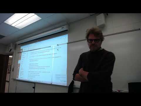
Andy Baker introduces sampling distributions as distributions of statistics produced by repeatedly taking samples, distinguishing them from distributions of raw observations. He explains how the sample mean’s center, shape, and spread relate to population properties, then calculates standard errors for sample means and proportions, including examples with population standard deviation 18 minutes and a proportion of 0.55.
Key takeaways
- A sampling distribution is formed by repeatedly calculating a statistic, such as x̄, and plotting those results; it is not the distribution of raw observations in one sample.
- The mean of the sampling distribution of x̄ equals the population mean μ in the theoretical model, so repeated sample means provide an unbiased center for estimating μ.
- The standard error of a sample mean is σ/√n; with σ = 18 minutes, it falls from 3.6 minutes at n = 25 to about 1.54 minutes at n = 136.
- The Central Limit Theorem makes the sampling distribution of the mean approximately normal for sufficiently large samples; Baker gives n > 30 as a general guideline for skewed populations.
- Random selection matters for representativeness: sampling only basketball centers or only point guards would bias an estimate of overall free-throw performance.
- For a proportion p = 0.55 from a sample of n = 100, the standard error √[p(1 − p)/n] is approximately 0.05.
Chapters
- Andy Baker previews Quiz 6 and recommends working through its sample questions before the next class.
- He frames the course as balancing quiz-ready problem solving with understanding why statistical methods work.
- He encourages students to ask for help and use AI as a learning aid rather than only copying answers.
- The class revisits five practice questions about populations, samples, parameters, and statistics.
- A population is the full group relevant to a research question, such as all IU Indianapolis undergraduates, not everyone in the world.
- Baker uses the commute-time example to distinguish all students from the 18 or 24 students in one class section.
- Capital N denotes population size, while lowercase n denotes sample size.
- A parameter describes a population, such as its mean μ or standard deviation σ; a statistic describes a sample.
- The sample mean is written x̄, sample standard deviation is s, and a sample proportion is written p̂.
- The standard deviation of a sample is s, while σ represents the population standard deviation.
- All IU Indianapolis students who commute form the population, while 36 poll respondents form a sample.
- A stated value of σ = 18 minutes describes the population, so it is a parameter.
- Earlier class material described entire populations; the next stage uses samples to infer population characteristics.
- Baker compares a representative sample to a Chick-fil-A nugget sample that should reflect the typical nugget, not an unusual one.
- The central question shifts to how accurately a study’s sample represents the broader population.
- Baker imagines a bag containing the integers 1 through 100 and repeatedly draws five numbers to calculate sample means.
- The population mean is 50, the midpoint of 1 through 100, and the first two example sample means are 70.2 and 28.4.
- Different samples produce different results, creating sample-to-sample variability, described informally as wobble or bounce.
- Each of 100 repeated draws contains five values, and each resulting x̄ is one statistic in the collection.
- The mean of the 100 sample means is approximately 48, close to the population mean of 50.
- Baker introduces μx̄ as the mean of the sampling distribution, which approaches μ as the number of repeated samples grows.
- A sampling distribution is the pattern formed by repeating a sample statistic many times, commonly displayed as a histogram.
- A sample distribution describes observations within one sample; a sampling distribution instead displays statistics such as many x̄ values.
- The example histogram contains sample means, not the individual numbers drawn from the bag.
- The sampling distribution’s center is the population mean μ, with repeated sample means averaging toward that value.
- Its spread measures how much sample means vary, and Baker introduces standard error as the relevant measure.
- For sample means, the standard error is σ divided by the square root of n, so larger samples produce less variability.
- The Central Limit Theorem says the sampling distribution of the mean becomes approximately normal when sample size is sufficiently large.
- Baker emphasizes random, unbiased sampling: selecting only basketball centers or only point guards would distort estimates of free-throw performance.
- A sample limited to seniors or first-year students may also fail to represent the full IU Indianapolis student population.
- If the population is already normally distributed, the sampling distribution of x̄ is normal for any sample size.
- For a flat population pattern, Baker gives roughly 10 to 15 observations as a rule of thumb for an approximately normal sampling distribution.
- For skewed data, he gives n greater than 30 as a general guideline; increasing n makes the distribution of sample means more bell-shaped.
- Standard error of the mean is the standard deviation of the sampling distribution of x̄, written SEₓ̄ or σₓ̄.
- With σ = 18 minutes and n = 25, the calculation is 18/√25 = 3.6 minutes.
- With σ = 18 minutes and n = 36, the calculation is 18/√36 = 3 minutes.
- For σ = 18 minutes and n = 136, Baker calculates 18/√136, approximately 1.54 minutes.
- The examples show standard error falling from 3.6 at n = 25 to 3 at n = 36 and about 1.54 at n = 136.
- A larger sample size reduces sampling variability, which is why studies with more observations can produce more precise estimates.
- For a sample proportion, the standard error is calculated as √[p(1 − p)/n].
- Using p = 0.55 and n = 100, the result is √[0.55 × 0.45/100], approximately 0.05.
- Baker says the next class will use standard errors in confidence intervals and begin with Quiz 6 practice problems; he confirms formulas will be available on the quiz.
Transcript excerpt
0:58 All right. 10:30. All right, let's roll. I don't know. Do I have Guess I probably
1:46 have graded quizzes. Yeah, I got grading quizzes. So, uh, I'll sprinkle those out as we go here so we don't waste too much time on that. All right. Um, [clears throat] Z tables in case we need it. Always need to carry the Z table with us. Okay. So, as a reminder, we've got quiz six next time we meet. Uh, and as you guys have said, you want at the beginning, so we'll get it at the beginning. Uh, quiz six is loaded. Keep in mind, we are being recorded. Make sure I'm on camera here. Looks good, right?
2:35 I don't know how good I don't know how much people are using these. I don't look at my views or anything. I hope y'all are anyhow. All right. So, quiz six. Just go ahead and take a look at it. You'll see there's already sample questions. So, there sample questions. Now, this is going to be a loaded one. Keep in mind, I did give you the 10 out of 10 on quiz five. So, I kind of gave you a little bit of grace. So, I I take it back in the terms in in terms of a lot of stuff on just one uh quiz here. So, it's September 24th, which almost seems like it was a month ago. uh and then you have online lecture three October 1st so our last lecture and today's lecture October 6. So a lot of stuff and I provide study questions from each of those and so when
3:24 we go through this particular course there's kind of yeah as I'm going I'm teaching this for the first time so I'm kind of thinking as I go and so for some
This is the start of the transcript. Save this video free for the whole transcript, searchable and time-coded.
Related notes
Summary, takeaways, and chapters were generated by AI from the video's transcript and may contain errors. The video belongs to its creator, Andy Baker.