Intro to Statistics at IU Indianapolis - Dispersion Lecture
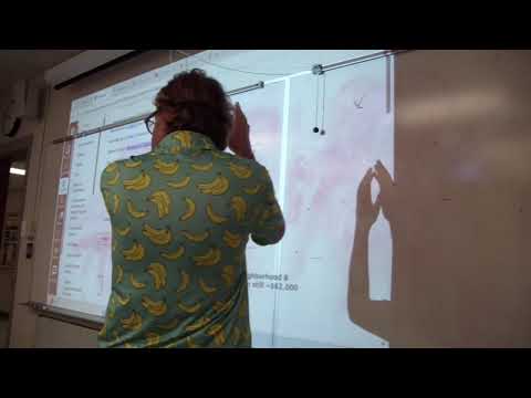
Overview
Andy Baker introduces four measures of dispersion, showing how range and interquartile range describe spread differently from variance and standard deviation. He explains when each measure is appropriate, distinguishes sample variance using n − 1 from population variance using N, and works through a sample of five study-hour values to obtain a variance of 7 hours squared and a standard deviation of about 2.65 hours.
Key takeaways
- Range is the maximum minus the minimum, making it quick to calculate but highly sensitive to outliers because only the two extremes determine its value.
- The interquartile range, Q3 − Q1, measures the spread of the middle 50 percent and is more informative than range when data are skewed or contain extreme values.
- Sample variance divides the sum of squared deviations from the mean by n − 1, while population variance divides by N.
- For study-hour values 2, 4, 4, 6, and 9, the mean is 5, the squared deviations sum to 28, sample variance is 7, and standard deviation is approximately 2.65 hours.
- Variance is expressed in squared units, so taking its square root yields standard deviation in the original units, such as hours.
- Skewness comparisons using the mean, median, and mode require quantitative data; nominal and ordinal categories do not support those calculations.
Chapters
- A left-skewed, or negatively skewed, distribution has mode greater than median, which is greater than mean.
- A right-skewed, or positively skewed, age distribution has mean above the median and mode because older outlying values pull the mean upward.
- Skewness based on mean, median, and mode applies to quantitative data, not nominal or ordinal categories whose bar positions are chosen rather than placed on a number line.
- Andy Baker notes that IU Anywhere can behave differently because it runs as a virtual desktop inside another desktop.
- For the reported SPSS screen issue, go to Utilities, open Control Panel, and choose End All to return to the expected screen.
- A screenshot of the problem helped identify that the student's screen differed from Baker's.
- Lab 2 is available, due Sunday, and includes a video tutorial demonstrating the SPSS click sequence.
- Quiz 2 covers the previous lecture and this dispersion lecture, lasts about 15 minutes, and is closed-book and closed-note.
- Students may use a writing utensil and a calculator, but not a phone; practice questions are expected to appear on the course page.
- A median alone can conceal major differences in spread, as illustrated by two neighborhoods with nearly identical median home values but very different home-price diversity.
- Dispersion describes how tightly values cluster or how far apart they are, complementing measures of what is typical.
- Baker connects dispersion to class data such as age, stress, and hours of sleep.
- Range equals the highest value minus the lowest value and is suitable for quantitative interval or ratio data, not nominal or ordinal data.
- For the sleep example, the range is 11 − 4 = 7 hours; for commute time, it is 40 − 0 = 40 minutes.
- Range provides a quick snapshot but depends entirely on the two extreme values, so it is not resistant to outliers.
- The interquartile range is Q3 − Q1 and summarizes the spread of the middle 50 percent of ordered data.
- For 21 sleep observations, Baker finds the overall median, then the lower and upper quartiles: Q1 = 5.5 and Q3 = 7.25.
- The resulting IQR is 7.25 − 5.5 = 1.75 hours, suggesting the central sleep values are relatively tightly clustered.
- Because extreme observations outside the middle half do not determine the IQR, it is resistant to outliers and useful for skewed data.
- Variance measures differences from the mean and, unlike range, uses every score in the data set.
- Baker describes variance as scaffolding: it is mainly calculated to produce the more interpretable standard deviation.
- The formula is provided for future quizzes, while students should focus on understanding its steps and keeping calculations organized.
- For a complete population, divide the sum of squared deviations by N; for a sample, divide by n − 1.
- Baker uses five selected students as an example of a sample, not the entire class population, so its denominator is 5 − 1 = 4.
- He presents n − 1 as the sample-variance rule and notes that its deeper rationale involves degrees of freedom.
- The sample consists of five study-hour values: 2, 4, 4, 6, and 9.
- Their total is 25, so the mean is 25 ÷ 5 = 5 hours.
- Each score is compared with the mean to find its deviation: −3, −1, −1, 1, and 4.
- The deviations sum to zero, so adding unsquared differences would not show overall spread.
- Squaring the deviations removes negative signs and gives greater influence to larger differences.
- The squared deviations are 9, 1, 1, 1, and 16, producing a sum of squares of 28.
- For the five-student sample, divide the sum of squares, 28, by n − 1 = 4 to get a sample variance of 7.
- Variance is measured in squared units, so this example produces 7 hours squared and is not usually the final quantity of interest.
- Standard deviation is the square root of variance: √7 is approximately 2.65 hours, returning the measure to the original units.
- Baker recommends the IQR for skewed data because it is resistant to extreme values, and standard deviation for roughly symmetrical data.
- Standard deviation is described as frequently used in sociology; range is a quick descriptive measure and is more common in some physical-science contexts, such as daily temperature highs and lows.
- All the dispersion calculations discussed require quantitative data; the next class will connect the mean and standard deviation.
Transcript excerpt
0:05 uh quizzes. I'll return those next time. So, I'll kind of get that pattern going as far as returning them on Thursdays. Why? Cuz that's when I know most people will be here for sure, for certain. All right. So, we are so I guess I'll go ahead and start here while I am here. Uh and so the measures of central tendency the last lecture uh the last lecture uh it's posted right here. So once again if there is ever an issue where you don't or aren't able to be here by today this is being recorded uh it will then be posted onto um the page that we're using today. And so that's there. And if you keep on scrolling down, you'll see that I went
0:53 ahead and I filled the table that I analyzed and discussed uh last time. And then I asked the question at the very end. First off, I asked you and I, you know, I assume no one did this, so I'm not going to be upset if it didn't happen, but some homework was to go ahead and populate the mode, median, and mean. Uh but with that being said, uh we can still see particular patterns. Uh so in this case here, this data here, I don't even know what it is. I don't even care what it is. But we see the mode is greater than the median and greater than the mean. So which one of these does that fit with? Where the mode is greater
1:40 than the median, which is greater than the mean. Boom. This one. See how mode alligator chomp toward the mode. So it means it's bigger than median which means it's bigger than me. So in this case don't even having to look at that I
This is the start of the transcript. Save this video free for the whole transcript, searchable and time-coded.
Related notes
Summary, takeaways, and chapters were generated by AI from the video's transcript and may contain errors. The video belongs to its creator, Andy Baker.