Spanning Trees
Overview
Kent Quanrud develops spanning-tree algorithms from graph definitions and counting arguments, then shows how duality between forests and spanning sets turns locally maximal or minimal solutions into global optima. For weighted graphs with distinct edge weights, he characterizes edges that belong to every minimum spanning tree and uses that property to justify Kruskal's, Borůvka's, and Prim's algorithms, including their main running-time bounds.
Key takeaways
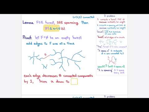
- In a connected graph, every forest has at most n minus 1 edges and every spanning set has at least n minus 1; with k connected components, the corresponding bounds are n minus k.
- A maximal forest is spanning because any edge joining two of its components could be added without creating a cycle; this converts a local stopping condition into a maximum-size forest.
- With distinct weights, an edge is good when every edge set connecting its endpoints contains a heavier edge; good edges belong to every minimum spanning tree.
- The lightest edge crossing any cut is good, providing the shared correctness certificate behind Kruskal's, Borůvka's, and Prim's algorithms.
- Kruskal's algorithm combines O(m log m) sorting with near-linear disjoint-set operations, while Prim with a Fibonacci heap runs in O(m + n log n) and Borůvka runs in O(m log n).
Chapters
- The motivating task is to connect every house in a town while minimizing total wire length.
- A solution needs to make every pair of houses mutually reachable, but adding a cycle is unnecessary because one cycle edge can be removed without disconnecting the network.
- The class uses this problem to develop algorithms for connecting graph vertices with minimum total edge weight.
- A circuit is a closed walk, a forest contains no cycles, and a tree is a connected forest.
- An edge set S spans an edge e when S connects the endpoints of e; S is spanning when it spans every graph edge.
- The two central unweighted goals are finding a forest with the most edges and a spanning set with the fewest edges.
- In a connected graph with n vertices, an acyclic edge set has at most n minus 1 edges.
- Start with n isolated vertices; each edge added without creating a cycle joins two components and reduces the component count by exactly one.
- The component count can fall only from n to 1, so at most n minus 1 such edge additions are possible.
- A spanning set starts with one connected component, and deleting a single edge can increase the component count by at most one.
- After all edges are deleted, n vertices form n separate components, so at least n minus 1 deletions were needed.
- For a graph with k connected components, applying the connected-graph bounds component by component gives at most n minus k forest edges and at least n minus k spanning edges.
- A maximal forest cannot accept another edge without creating a cycle, while a maximum forest has the greatest possible number of edges.
- A minimal spanning set cannot lose an edge and remain spanning, while a minimum spanning set has the fewest possible edges.
- The distinction is between a locally unextendable or irreducible solution and a globally optimal one.
- If a maximal forest does not span the connected graph, an unspanned edge can be added without creating a cycle, contradicting maximality.
- If a minimal spanning set contains a circuit, removing any circuit edge preserves connectivity, contradicting minimality.
- A forest that spans is therefore a tree with n minus 1 edges; the complementary minimal-spanning-set argument also yields a tree.
- The weighted objective is a minimum-weight spanning tree, with distinct edge weights assumed to simplify the arguments.
- An edge e is called good when every edge set spanning e contains another edge heavier than e.
- Equivalently, e is not the heaviest edge on any circuit; the lecture aims to connect this property to membership in every minimum spanning tree.
- If e belongs to every minimum spanning tree but is heavier than all edges in some set spanning it, removing e splits a tree into two components.
- That spanning set must contain an edge crossing the split; replacing e with that lighter edge produces a lighter spanning tree, a contradiction.
- Conversely, if e is good but absent from a minimum spanning tree, the tree's path between e's endpoints contains a heavier edge that can be swapped out for e.
- For any edge set H, consider the components it induces and the graph edges whose endpoints lie in different components.
- The minimum-weight edge crossing those components is good: any edge set spanning it must cross the same separation with another edge.
- This cut-based lemma provides a certificate for safely adding an edge to a minimum spanning tree.
- Kruskal's algorithm sorts all m edges by weight and considers them from lightest to heaviest.
- It adds an edge only when its endpoints are in different components, keeping the selected edges acyclic.
- For an edge considered at a given point, the previously processed edges form a certificate that it is the minimum edge crossing the relevant components.
- Prim's algorithm begins at any vertex and repeatedly adds the lightest edge leaving the growing tree.
- Treat the tree as one component and all vertices outside it as the other; the selected edge is the lightest edge crossing that cut.
- The cut certificate makes every chosen edge good, so the process grows a minimum spanning tree.
- Kruskal needs to test whether each edge's endpoints are already in the same connected component.
- A disjoint-set union structure supports component unions and same-set queries, with total operation cost near-linear in m plus n times the inverse Ackermann function α(n).
- Because α(n) grows extremely slowly, sorting the edges, typically O(m log m), is the dominant cost.
- In each Borůvka round, every current component selects its cheapest outgoing edge, and the selected edges are added together.
- Each round reduces the number of components by at least a factor of two, giving O(log n) rounds.
- Scanning the graph in each round gives an O(m log n) running time; the method is also naturally parallelizable.
- Kruskal and Borůvka run in O(m log n) time under the lecture's standard graph-size assumptions.
- Prim with a Fibonacci heap takes O(m + n log n), using repeated minimum-edge extraction and heap updates.
- The lecture briefly notes faster MST results, including a randomized O(m + n) algorithm, but focuses on the three core methods.
Transcript excerpt
0:04 Um okay. So yeah. All right. So today we're doing spanning trees and uh we're actually leaving well it'll always be around all this MP completeness and this risk of heart problems but we're also going to be doing a lot more algorithms and how to solve problems and stuff as well. Okay. So so we sort of already hit the peak. I I I mean I think that the MP completeness stuff is probably the deepest stuff just to wrap your mind around and getting used to showing problems are hard instead of just solving them. At least for me, this kind of reverse thinking, it just takes some time to get used to. That's one reason we do a little earlier in the class compared to other classes is to actually give you more time to digest uh uh the materials. But this this might look a little bit more like stuff we were doing before midterm one. So here's the the the basic setup. In fact, this was the
0:52 historical uh motivation apparently in like the 1800s. Um, okay. So, uh here's like a town. I'm really good at drawing houses. And uh you want to connect the town with electricity. Okay. So, you want to connect them with wires. And um let's say like the amount of wire is basically proportional to the length on the on the on the board. Okay. So, so your goal is to choose kind of the the minimum total amount of wire uh to connect all the houses together. That make sense? >> Yeah. Fully connected. So, every house should be able to reach each other like it's, you know, like as if they're all using the same electrical source. >> Yeah.
1:40 >> Or data center, whatever is the There is an algorithm. Yeah, this we're
This is the start of the transcript. Save this video free for the whole transcript, searchable and time-coded.
In this course
Related notes
Summary, takeaways, and chapters were generated by AI from the video's transcript and may contain errors. The video belongs to its creator, Kent Quanrud.