CS 181 Lecture 12 -- Fall 2026, UCLA
Overview
Eli Jaffe uses a Turing machine for palindrome recognition to show how a finite-state machine can manipulate a tape, then explains why Turing machines can simulate programming languages and machine variants. The lecture introduces the Church-Turing thesis, the universal Turing machine, and a binary encoding of transition tables as groundwork for proving that some functions are uncomputable.
Key takeaways
- Palindrome recognition needs only a fixed number of states because the machine remembers one bit at a time, marks processed symbols on the tape, and compares matching positions from opposite ends.
- The lecture states that a single-tape Turing machine can simulate a Python program taking T steps with about T squared steps of overhead, despite lacking Python's direct variables, loops, and random access.
- Adding multiple tapes or heads changes efficiency but not which functions are computable: the lecture describes multi-tape simulation on one tape and gives a T log T overhead for a two-tape simulation.
- The Church-Turing thesis claims that every function computable by physical means is Turing-computable; quantum computing may improve efficiency without expanding the set of computable functions.
- The universal Turing machine is possible because a transition table can be encoded as binary data, allowing a fixed machine to interpret another machine's description and input.
- Universal evaluation and uncomputability rely on the same code-as-data idea: machine descriptions can be encoded and processed, enabling proofs about both simulation and fundamental limits.
Chapters
- Homework 4 is due November 21 at 9:59 p.m.; Exam 2 is scheduled for November 23.
- Eli Jaffe announces no class on Veterans Day and adds Monday office hours alongside Zoom office hours.
- The technical focus is a Turing machine for palindromes, followed by results about computational power and limitations.
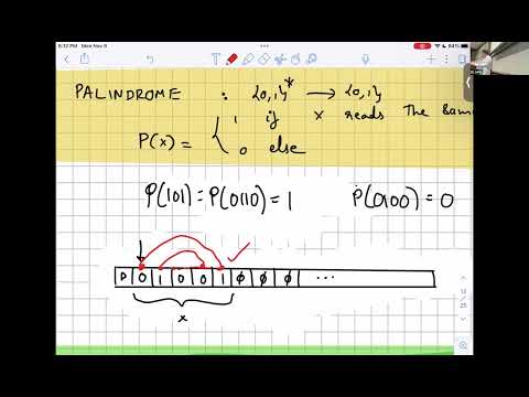
- The palindrome function outputs 1 when a bit string reads identically forward and backward, such as 101 or 0110.
- The example 0100 is not a palindrome and should produce 0.
- The machine must use local tape reads, head movement, and a finite transition table to compare the string's ends.
- The proposed strategy remembers the first bit, travels to the input's end, and compares it with the last bit.
- If the bits match, the machine marks both as processed and repeats with the next unprocessed pair.
- A mismatch immediately establishes that the input is not a palindrome.
- The machine stores whether the first bit was 0 or 1 in one of a fixed number of states.
- It overwrites a processed input bit with a marker such as A, avoiding the need for a state per input position.
- A special end marker, shown as B in the explanation, lets the machine detect the input boundary and move back to the last bit.
- After a matching comparison, the machine replaces the matched final bit with an end marker and returns toward the first unprocessed bit.
- The next round begins by locating the first A marker and moving to the next unseen input symbol.
- If every pair matches, the machine cleans the tape and outputs 1; any mismatch leads to output 0.
- Jaffe traces an input beginning 0101100 and shows the machine marking symbols, storing a bit in its state, and comparing opposite ends.
- The sample eventually finds a 1-to-0 mismatch and enters a reject state that writes 0.
- A Turing machine simulator demonstrates the same process, using blank symbols instead of A markers.
- Python offers variables, functions, loops, conditionals, recursion, data structures, and random access directly.
- A basic Turing machine instead reads and changes one tape cell at a time, with a finite set of states and symbols.
- The palindrome example establishes the expected description level: explain local scans and tape changes rather than writing every transition.
- The lecture states that a Turing machine can simulate programs with features such as loops, recursion, and random access.
- For a Python computation taking T operations, the stated single-tape simulation overhead is about T squared steps.
- The quadratic overhead is presented as surprisingly small given how much more constrained a Turing machine appears.
- Alan Turing introduced Turing machines in 1936 and also contributed to mathematical logic, statistics, and wartime codebreaking.
- The lecture connects his work on the Enigma codebreaking effort with ideas related to mechanical computation.
- The question becomes whether adding heads, tapes, or other capabilities can compute functions that a standard machine cannot.
- A multi-head machine can be simulated by a standard single-head Turing machine.
- A machine with multiple tapes can also be simulated on one tape, though the lecture describes two tapes as reducing simulation overhead to about T log T.
- A tape infinite in both directions is described as equivalent in computational power to a two-tape machine.
- The Church-Turing thesis says every function computable by physical means is computable by a Turing machine.
- It is a thesis rather than a theorem because physical computability is an empirical claim, not a formal definition that can be proved from the machine model.
- Quantum computers may improve efficiency, but the lecture says they do not compute functions beyond those computable by Turing machines.
- Jaffe introduces the HOCAET principle, short for “have our cake and eat it too,” for switching between high- and low-level descriptions.
- To prove a function computable, a Python program can serve as a concise construction because Turing machines can simulate it.
- To prove a function uncomputable, the more precisely constrained Turing-machine model provides a useful target for impossibility proofs.
- During the break, Jaffe addresses a question about using the same symbol for a language and its associated function, recommending confirmation with the grader.
- A student asks what motivated the progression from circuits to finite automata and then Turing machines.
- Jaffe describes the progression as fixing limitations exposed by larger inputs and new computational needs, while noting that he wants to investigate the history further.
- A universal machine takes another machine's description and an input, then simulates that machine on the input.
- Unlike the universal-circuit result discussed earlier, the universal Turing machine has no fixed bound on the size of the machine it can simulate.
- The universal-machine theorem is presented as a provable result, unlike the Church-Turing thesis.
- Universal simulation requires treating a machine's description as data that can be placed on another machine's tape.
- A transition table with k states and L symbols has one row for each state-symbol pair, for k times L rows.
- Each transition records the current state and symbol, next state, symbol to write, and head action.
- States and tape symbols can be represented by integers, and head actions can be encoded as 0 for left, 1 for right, 2 for stay, and 3 for halt.
- The transition table is serialized row by row as five-integer tuples, preceded by the machine's state and alphabet counts.
- A machine with k states and L symbols therefore has k times L transition tuples.
- The integer list is converted to a bit string using prefix-free integer encodings so the boundaries between values remain identifiable.
- The notation ⟨M⟩ denotes the binary encoding of a Turing machine M; invalid encodings are conventionally treated as machines that output 0.
- The evaluation function takes a machine encoding and input, and represents either the machine's output or nontermination with a special symbol.
- Alan Turing's 1936 result establishes that a Turing machine can evaluate other Turing machines from their descriptions.
- A universal machine is a fixed machine with a finite transition table, yet it can simulate machines of arbitrary size.
- Jaffe notes that universal machines can use as few as 25 states and four symbols, and previews next lecture's analysis of uncomputable functions.
Transcript excerpt
0:04 All right. Uh, let's get started. Hello everybody. Welcome back. Um, last time on Dragon Ball Z, we defined touring machines, which is very, very exciting. We reached a pivotal moment in the course. And we also showed a couple examples of languages that were computable by touring machines, defined what it means to be computable by touring machines. We specifically looked at majority. Actually, I think that was the only one we looked at uh and gave this cool algorithm, saw it play out on that touring machine simulator. And today we are going to be diving a little bit deeper and we're going to
0:52 look at one more example of how a touring machine plays out, how it computes things, what's actually going on and then we are going to talk about the power and limitations of touring machines as a programming language as a computational model. Um, before we jump into that, a couple logistical announcements. That's too big. Uh, first of all, as you all hopefully know, homework read is due tonight at 9:59 p.m., which I can only assume that's where all your classmates are.
1:42 They're at home busy working on their homework. Um, I actually I decided to release homework 4 a little bit early because I was like, why why gatekeep the homework? You know, if people want to start it early, like let them start it early. So, homework 4 is out now and it's not due in a week. It's due uh on November 21st at 9:59 p.m. So, that's in like a week and a half or so. Um, and I think that's like two days before our next exam. So, our exam two is going to be on 11:23. Same deal as last time. And two other minor logistical
This is the start of the transcript. Save this video free for the whole transcript, searchable and time-coded.
In this course
Related notes
Summary, takeaways, and chapters were generated by AI from the video's transcript and may contain errors. The video belongs to its creator, Eli Jaffe.