UUtah Data Mining | Fall 2026 | L21 : Anomaly Detection
Overview
Anomaly detection is framed as a three-part task: model what data to expect, define a constrained family of anomaly shapes and search it, then test whether the best-scoring region is genuinely unusual. For an IID Gaussian model with known standard deviation, a log-likelihood ratio compares separate mean fits inside and outside a candidate subset against one fit to all observations; for time-series change points, candidate intervals can be scanned efficiently by updating running statistics. The lecture distinguishes coherent anomalous regions from scattered outliers and discusses significance checks using approximate likelihood-ratio thresholds, simulated baseline data, and permutation tests.
Key takeaways
- A useful anomaly detector needs three explicit components: a baseline data model, a constrained family of candidate subsets, and a test of whether the best score is statistically unusual.
- For IID Gaussian observations with known standard deviation, the log-likelihood ratio compares the squared-error fit from separate subset and complement means with the fit from one overall mean.
- Anomaly shape determines the question being answered: a contiguous time-series interval captures a change-point event, while selecting scattered extremes primarily detects outliers.
- A one-dimensional change-point scan can run in linear time because moving the candidate boundary changes only one observation's membership, allowing running sums and squared-error statistics to update incrementally.
- A log-likelihood-ratio threshold near 2 is only an approximate 0.05-significance guide under suitable assumptions; simulation from a fitted baseline or permutation of observed values can provide data-driven score thresholds.
Chapters
- The anomaly-detection lecture introduces a broad topic through one tractable mathematical example.
- A 50-point homework assignment is due the following Tuesday and applies the lecture's scoring and outlier concepts.
- The lecture organizes anomaly detection around modeling expected data, constraining anomaly shape, and assessing statistical significance.
- A candidate anomaly is a subset of observed data X, or equivalently a region in the data's feature space.
- The goal is to identify a jointly unusual subset, rather than simply rank individual observations by extremeness.
- The distinction matters because a group can be unusual collectively even when each point looks plausible on its own.
- The framework assumes observations X₁ through Xₙ are IID from an unknown model of the world.
- A parameterized probability distribution provides a likelihood for judging how well a candidate model explains the data.
- The IID assumption allows the joint likelihood to be formed from individual observation likelihoods.
- A shape family specifies which subsets are eligible, preventing arbitrary selection of the most extreme observations.
- For a one-dimensional density, an interval could capture a localized excess or bump in observations.
- The family must encode coherent structure, such as contiguous time points, rather than allow unconstrained gerrymandering.
- Step one defines a probability-based score for candidate subsets; step two searches the allowed shapes for the highest score.
- Step three tests whether the winning subset is unusually strong, since an optimizer always returns a best candidate.
- A maximum-scoring region is not automatically significant; it may be the least ordinary pattern in otherwise routine data.
- For IID data, the likelihood of the full dataset is the product of the likelihoods of X₁ through Xₙ under parameter θ.
- The maximized likelihood chooses the parameter value that best fits the observations.
- The anomaly score compares separate maximized likelihoods for a subset S and its complement against one maximized likelihood for all of X.
- The worked model is Gaussian with unknown mean μ and known standard deviation σ.
- A Gaussian density is not the probability of observing one exact continuous value, which is zero; it is a density that integrates to one.
- The normalizing constant can be omitted in likelihood comparisons when it is identical across the models being compared.
- Taking the natural logarithm converts the product of Gaussian likelihood terms into a sum over observations.
- With known σ, the log-likelihood is proportional to the negative sum of squared deviations from μ.
- Log-likelihoods are easier to calculate numerically than products of many small exponential terms.
- Maximizing the Gaussian log-likelihood over μ is equivalent to minimizing the sum of squared errors.
- The minimizing estimate μ* is the arithmetic mean of the observations in the fitted dataset.
- The closed-form mean makes it straightforward to refit the baseline and candidate subsets.
- The log-likelihood ratio adds the log-likelihood for S to that for X outside S, then subtracts the log-likelihood for all of X.
- For the Gaussian example, the three terms correspond to squared-error fits using the mean inside S, outside S, and across all data.
- A larger ratio indicates a greater improvement from fitting the two regions separately, and sign conventions must preserve that direction.
- The running example assigns each observation Xᵢ to a time point and compares a candidate region's mean with the outside mean.
- The score reflects how much separate fits reduce squared error relative to one overall mean.
- When the variance is shared and known, its common coefficient cancels in the likelihood ratio.
- Scattered extreme points, such as three isolated values, are treated as outliers rather than one coherent event.
- A contiguous block with a changed prevailing pattern is an anomalous region and can represent a change point.
- The shape constraint encourages the method to find meaningful events instead of merely selecting the ten largest values.
- A candidate subset can be defined as the observed data intersected with a region R from an allowed shape family.
- For time series, candidate shapes include intervals; a one-sided interval represents a change point.
- Spatial searches can use circles, rectangles, or census regions, while classifier searches can use half-spaces that favor positive over negative examples.
- A candidate change point t defines a one-sided region, and the algorithm evaluates its log-likelihood ratio across possible t values.
- As t advances by one observation, only one point changes sides, so running counts, sums, means, and squared-error terms can be updated.
- With these incremental calculations, the simple time-series scan can find the best change point in linear time.
- The best region always exists computationally, so its score needs a separate significance assessment.
- Under suitable statistical assumptions, the lecture gives a log-likelihood-ratio value around 1.96, or roughly 2, as an approximate 0.05-level guide.
- The threshold depends on the desired significance level and the model assumptions, so the value near 2 is a heuristic rather than a guarantee.
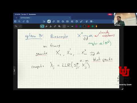
- Parametric resampling generates M synthetic datasets, each with n observations drawn from the fitted baseline distribution, and reruns the anomaly search.
- The resulting score distribution supplies an empirical cutoff, such as its upper 5 percent, for comparison with the original dataset's score.
- A permutation test instead shuffles the time-series values while retaining their positions as a reference for scores under disrupted temporal structure.
- Results far beyond the simulated or permuted threshold are more persuasive than scores close to the cutoff.
Transcript excerpt
0:26 That's great. So, welcome back everyone. So, let's get started. Um, so today we're going to be talking about anomaly detection. Um, this is a potentially kind of huge area and I could spend probably the whole semester on this. We're going to spend oh, one lecture on it. Uh, so I'm going to go through what I believe is a very clean example of this that's going to kind of pull out a lot of the major um, so ideas you need to keep in mind. Um, but it's going to be a very clean example. So, we're going to kind of go through like all the math on this and you're going to kind of see the patterns that you sort of see in math, but know that it can be much more complicated than than than what we'll see today. Um,
1:17 so, so before we get into it, um, let's look at the schedule. Um, where are we? Okay, so we're in the noise section of the class and there's a new homework that's posted. It's due next week, Tuesday. Um, so it's posted online. There was an announcement on on Canvas about it. You should be able to do basically I think all of it after today's lecture. Um it's pretty short. It's only worth 50 points, not the typical 100 points. So it's about half of a regular assignment. Um it'll kind of be just exploring this sort of stuff we talked about today and then looking for outliers and stuff like this. So give you some practice doing it so you
2:06 feel comfortable with the math that we're going through today. Um um okay. So this is due in a week. The other half of this assignment will be due at the end of the semester. Okay. So
This is the start of the transcript. Save this video free for the whole transcript, searchable and time-coded.
In this course
Related notes
Summary, takeaways, and chapters were generated by AI from the video's transcript and may contain errors. The video belongs to its creator, UofU Data Science.