STAT 638 (Fall 2026), Lecture 22

Overview

Samiran Sinha develops Bayesian linear regression from its mathematical foundations through practical R workflows: completing the square yields normal posterior forms, while rstanarm and brms demonstrate fitting, diagnostics, and posterior prediction. He then codes a Gibbs sampler for a g-prior model, examines suspiciously narrow results, and introduces Bayesian model selection through posterior model probabilities and model averaging.

Key takeaways

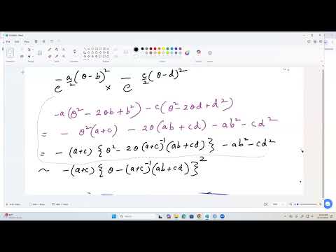
Multiplying normal-kernel terms adds their precision matrices: the combined covariance is (B+D)⁻¹ and the posterior mean is (B+D)⁻¹(Ba+Dc).
An R-hat near 1 assesses agreement across chains, while effective sample size and autocorrelation describe sampling efficiency; satisfactory convergence does not guarantee independent-looking draws.
In the rstanarm example, four chains of 3,000 iterations yield 12,000 total iterations, but a 50% warm-up leaves about 6,000 draws for posterior summaries.
Posterior prediction at a chosen covariate profile combines uncertainty in regression parameters with outcome-level randomness by repeatedly drawing parameters and then future outcomes.
The g-prior Gibbs sampler uses normal and inverse-gamma full conditionals; its implausibly narrow intercept interval at g=100 motivates checking implementation, prior sensitivity, and convergence across multiple chains.
Bayesian model comparison can either select the model with the largest posterior probability or average inference across models using those probabilities as weights.

Chapters

0:00 Bayesian Regression: Likelihood, Priors, and Posterior Summaries

Sinha frames Bayesian inference around the likelihood and prior, which combine to form a posterior distribution.
Posterior distributions support parameter summaries, posterior predictive distributions, and model checks such as marginal likelihood calculations.
Linear regression provides a foundation for extending the same reasoning to binary, count, and categorical outcomes.

4:00 Completing the Square for Scalar and Vector Normal Kernels

For scalar normal-kernel terms, combining precisions gives posterior variance 1/(A+C) and mean (AB+CD)/(A+C).
For vector parameters, the corresponding covariance is (B+D)⁻¹ and the mean is (B+D)⁻¹(Ba+Dc).
Vector algebra requires careful matrix ordering; Sinha emphasizes that scalar factors can commute but matrices generally cannot.
The same square-completion result underpins normal regression models with multiple coefficients.

15:00 Classical Regression Tests and the rstanarm Model Setup

In classical regression, a coefficient’s t statistic and p-value assess the null hypothesis that the coefficient equals zero.
Sinha introduces rstanarm's stan_glm for a Gaussian linear model, with normal(0, 10) priors on coefficients and the intercept.
The example uses four MCMC chains and 3,000 iterations per chain; the prior for the residual scale is left to the package default.

17:00 Comparing Bayesian Estimates and Interpreting MCMC Output

The rstanarm output reports posterior means, including an intercept near 34.5 and a walk-time coefficient near −0.2, broadly resembling the classical estimates.
Sinha notes that flexible priors often yield estimates similar to classical results when model assumptions are reasonable.
Four chains of 3,000 iterations produce 12,000 total draws; after an apparent 50% warm-up, about 6,000 draws remain for summaries.
Effective sample size measures sampling efficiency: low values, such as about 1,725 for sigma, indicate substantial autocorrelation.

23:00 Trace Plots and Autocorrelation Reveal Slow Sigma Sampling

Trace plots help assess whether MCMC chains explore the posterior; tightly linked successive sigma draws indicate slow movement.
Sinha compares sigma traces with coefficient traces and recommends an autocorrelation function (ACF) plot when the difference is not visually clear.
High autocorrelation reduces effective sample size and estimator efficiency, even when a chain can still represent the target posterior.

28:00 R-hat Checks Convergence, Not Sampling Efficiency

The Gelman–Rubin R-hat statistic compares between-chain and within-chain variability across parallel chains.
R-hat near 1 indicates that chains have mixed toward the same posterior; Sinha gives 1.01 or lower as a practical convergence target.
A chain can have R-hat near 1 yet remain highly autocorrelated: convergence and efficient exploration are distinct diagnostics.

30:00 Posterior Predictive Checks at Specific Predictor Values

A posterior predictive check compares replicated outcome distributions with the observed distribution while conditioning on explanatory-variable values.
Sinha illustrates predictions for two covariate profiles: weight 150, age 46, walk time 10, heart rate 90; and weight 160, age 49, walk time 20, heart rate 130.
For each profile, posterior draws produce a predictive distribution summarized by its median and 2.5th and 97.5th percentiles.
To generate predictions conceptually, draw parameters from the posterior, then draw a future outcome given those parameters and the chosen predictors; repeat many times.

37:00 brms, NUTS, and Sampling from Complex Posteriors

Sinha compares the brms fit with the earlier rstanarm results and reports broadly similar estimates.
brms uses the No-U-Turn Sampler (NUTS), an MCMC method suited to sampling from complex, nonstandard posterior distributions.
He advises checking package defaults, including the prior on sigma squared, rather than assuming an unspecified prior.

40:00 Coding a G-Prior Gibbs Sampler and Investigating an Anomaly

The custom G-prior sets beta to a multivariate normal with mean zero and covariance proportional to g sigma²(XᵀX)⁻¹, with an inverse-gamma prior on sigma².
The full conditional distributions are multivariate normal for beta and inverse-gamma for sigma², enabling Gibbs sampling.
Sinha samples beta using a Cholesky factor and standard-normal draws; he notes that this approach may matter more when the coefficient dimension is around 1,000 than when it is only four or five.
With g set to 100, the intercept is about 24.34 with an unusually narrow interval of roughly 24.34–24.58, unlike estimates around 33–35 elsewhere; he suggests varying g, checking the code, and running multiple chains to inspect R-hat.

46:00 Bayesian Model Selection: Posterior Probabilities and Averaging

For candidate models Mₖ with parameter vectors θₖ, the marginal likelihood integrates the model likelihood over the prior on θₖ.
Posterior model probability is proportional to the prior probability of Mₖ multiplied by its marginal likelihood.
One option selects the model with the highest posterior probability; another averages the posterior distribution of a quantity of interest across models, weighted by their posterior probabilities.
Sinha closes by previewing specific model-selection methods for linear regression in the next lecture.

Summary, takeaways, and chapters were generated by AI from the video's transcript and may contain errors. The video belongs to its creator, Samiran Sinha.