STAT 638 (Fall 2026), Lecture 21

Overview

Samiran Sinha reviews Bayesian inference for a normal mean, develops Gibbs sampling for a four-location hierarchical model, and introduces the g prior for Bayesian linear regression. He compares standard Gibbs updates with a marginal-posterior sampling strategy to reduce autocorrelation, then applies the regression setup to simulated data modeled on a study of oxygen uptake in 54 male runners.

Key takeaways

When normal observations have known variance, the sample mean and sample size contain the information needed for inference about the population mean; extra summaries such as the sample minimum and maximum do not affect the posterior.
In the four-location lead model, each θᵢ update combines within-location evidence with the shared mean μ, while μ pools information across all four location parameters.
Posterior threshold probabilities such as P(θ₁ > 1.2 | data) can be estimated directly from Gibbs output by counting the fraction of sampled θ₁ values above 1.2.
The g prior uses the design matrix through covariance gσ²(XᵀX)⁻¹; choosing small g strengthens shrinkage toward zero, whereas large g weakens prior influence.
Marginalizing β allows direct sampling of σ² from its posterior given the data, followed by β conditional on σ², avoiding the iteration-to-iteration dependence of ordinary alternating Gibbs updates.
For the runner example, simulated coefficients are known only because Sinha generated the data; the intended real-world workflow estimates regression effects from observed outcomes and predictors without knowing how the data were generated.

Chapters

0:00 Quiz Corrections: Fixing the Probability Question

Sinha apologized for errors in the last quiz and awarded everyone full credit for Question 1 because its wording was incorrect.
The intended question asked which expression equals the posterior probability that the unknown mean μ exceeds 1.5 given the full dataset.

3:00 Known-Variance Normal Models and Sufficient Statistics

For 16 normal observations with known variance, the sample mean is sufficient for inference about μ; the individual observations can be reduced to their mean.
The quiz’s sample variance and minimum and maximum observations were unnecessary once the sample mean, sample size, and known population variance were available.

7:00 Completing the Square for the Posterior of μ

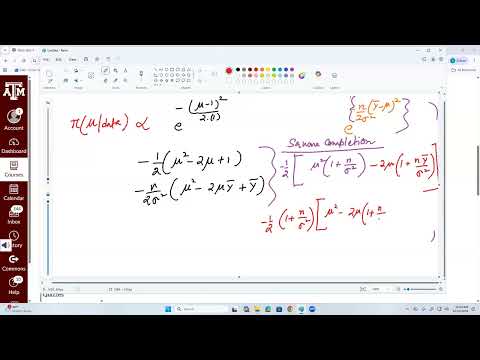
Sinha combines a normal prior with the normal likelihood and completes the square to obtain a normal posterior for μ.
The posterior mean depends on the prior information, sample mean, sample size, and known variance; the posterior variance depends on prior precision and sample precision.
For the quiz’s threshold probability, he evaluates the upper tail above 1.5 using the posterior mean and the square root of the posterior variance.

14:00 Four-Location Lead Study as a Hierarchical Model

The example models lead measurements at four water-sampling locations: observations have variance 0.09, location means θᵢ have variance 0.16 around μ, and μ has prior N(1.5, 0.25).
The target includes probabilities such as P(θ₁ > 1.2 | data), requiring inference across four location-specific means and the shared mean μ.

18:00 Deriving Gibbs Updates for Location Means θᵢ

The model has five unknown parameters—θ₁, θ₂, θ₃, θ₄, and μ—so Sinha proposes Gibbs sampling from each parameter’s full conditional distribution.
Each θᵢ conditional is normal, combining its location’s sample mean and sample size with the N(μ, 0.16) group-level distribution and the observation variance 0.09.

24:00 Updating the Shared Mean and Estimating Threshold Probabilities

The full conditional for μ is normal, combining its N(1.5, 0.25) prior with the four location means, whose shared-level variance is 0.16.
After repeatedly sampling θ₁ through θ₄ and μ, estimate P(θ₁ > 1.2 | data) or P(μ > 1.2 | data) by the proportion of retained draws above each threshold.
Sinha notes that real projects also require data curation and model selection rather than receiving a fully specified model and prepared group summaries.

30:00 Bayesian Linear Regression: Conditional Distributions

With normally distributed regression noise, the classical least-squares and maximum-likelihood estimates coincide; Bayesian inference also relies on the normal likelihood.
The preceding regression setup uses a normal conditional distribution for β and an inverse-gamma conditional distribution for σ², which can be sampled in Gibbs updates.

33:00 The g Prior Shrinks Regression Coefficients

Sinha defines the g prior as β | σ² ~ N(0, gσ²(XᵀX)⁻¹), using the known design matrix X rather than treating covariates as random observations.
A common choice is g = n, called the unit-information prior; the posterior mean shrinks the least-squares estimate β̂ by g/(g+1).
Small g pulls coefficients toward zero, while g tending to infinity makes the prior’s influence negligible.

37:00 Reducing Gibbs-Chain Autocorrelation by Marginalizing β

Ordinary alternating Gibbs updates for β and σ² link adjacent iterations, creating autocorrelation that can increase the variance of Monte Carlo estimates.
An alternative is to sample σ² directly from its marginal posterior given the data, then sample β conditional on that σ²; integrating β out removes dependence between successive joint draws.
Under the g prior, the marginal posterior for σ² is inverse-gamma, and the joint posterior for (β, σ²) is normal-inverse-gamma, enabling direct sampling.

45:00 Oxygen-Uptake Regression Example and Inference from Observed Data

Sinha introduces simulated data modeled on a 1994 study of 54 male runners, with maximal oxygen uptake as the outcome and weight, age, one-mile walk time, and post-walk heart rate as predictors.
Because the original data were unavailable, he simulated an illustrative dataset; in real analysis, the data-generating process and true coefficients are unknown.
The goal is to fit linear regression and infer its coefficients from the observed dataset; the next lecture will examine Bayesian analysis with independent priors.

Summary, takeaways, and chapters were generated by AI from the video's transcript and may contain errors. The video belongs to its creator, Samiran Sinha.