Scaling laws + exam review

Overview

Mohit Iyyer reviews the 40-question, handwritten-cheat-sheet exam and then explains how scaling laws use small-model experiments to predict language-model loss and choose model size and training data under a compute budget. He derives the approximate training-cost formula 6ND, describes the Chinchilla finding of about 20 training tokens per parameter, and explains why inference costs can favor smaller models trained on more data.

Key takeaways

The exam contains 40 equally weighted four-choice questions, allows only a handwritten two-sided 8.5-by-11-inch cheat sheet, and covers material through the scaling-laws lecture.
A simplified transformer training estimate is 6ND FLOPs: about 2N for forward computation and 4N for backpropagation per token, across D tokens.
Chinchilla’s compute-optimal rule of thumb is about 20 training tokens per parameter; its 70-billion-parameter model trained on 1.4 trillion tokens outperformed the larger, undertrained GPT-3.
Scaling laws estimate loss by fitting results from many smaller models across parameter counts and data sizes, then extrapolating; accuracy depends on experiment coverage and fit quality.
The best compute allocation for pretraining may differ from the best production allocation: high inference volume can make a smaller model trained on more data cheaper to serve.

Chapters

0:00 Exam Format: 40 Multiple-Choice Questions and a Handwritten Cheat Sheet

Exam 1 has 40 questions, each with four options and one correct answer, and uses the full class period.
Questions are equally weighted, so Mohit Iyyer advises moving on rather than spending ten minutes on one item.
Students may bring a handwritten cheat sheet on both sides of one 8.5-by-11-inch sheet; typed, printed, and electronic notes are not allowed.
Phones, laptops, and calculators are unnecessary, and students must stop when time is called.

4:57 Practice Question Types: Attention Windows, Perplexity, and Nonlinearities

A local attention mask with a window of eight tests whether students can reason about how receptive fields expand across transformer layers.
A question where training perplexity falls while test perplexity rises tests understanding of model quality and overfitting.
A transformer without nonlinearities collapses to a single linear transformation, a concept students should apply to modified scenarios.
Questions range in difficulty and may require extrapolating class concepts to situations not covered exactly in lecture.

7:57 Exam Coverage: Mixture of Experts, Attention Masks, and KV Caches

New exam topics include mixture-of-experts models: total versus active parameters, routing, and why sparse models can be preferable to dense models.
Students should review block attention masks and loss masking, including how mask changes affect model behavior.
This year emphasizes position encoding less: RoPE and ALiBi are not required, but the no-position-encoding approach discussed in class is relevant.
Review KV-cache growth and the difference between prefill and decoding, along with their effects on inference speed and memory.

13:37 Why Scaling Laws Matter: Predicting Results Before Expensive Training Runs

The broad empirical pattern is that larger models trained on more data tend to outperform smaller ones, often achieving lower perplexity.
Training frontier-scale models can cost billions of dollars and requires large GPU fleets and specialized engineering.
Scaling laws aim to use cheaper, smaller-model experiments to predict how model size and data choices will perform at larger scales.
OpenAI introduced early scaling-law work, while Google’s Chinchilla research later refined the compute-optimal allocation of parameters and data.

18:37 Emergent Abilities: Task Performance Versus Training Compute

A 2022 Google study plotted pretrained-model task accuracy against training FLOPs, with scale in that comparison largely tracking model size.
Tasks such as word unscrambling, Persian question answering, and multitask language understanding showed sharp apparent gains at larger scales.
The paper described abilities as emergent when they were absent in smaller models and became observable at larger scales.
Researchers debate whether these jumps reflect truly sudden capabilities or evaluation metrics that hide gradual improvements.

24:52 Training Loss, Downstream Tasks, and Generalization

A later study examined downstream performance against training loss and found that lower-loss models tended to do better on trivia, math, and multiple-choice tasks.
The plotted models ranged from about 1.5 billion to 32 billion parameters, with larger models generally reaching lower losses.
Next-token prediction acts like multitask learning: predicting a capital requires stored facts, while unfamiliar arithmetic requires learning a procedure.
Scaling can improve both memorization and generalization, but robust behavior on new examples depends on more than memorizing frequent answers.

30:39 Scaling-Law Variables: Parameters, Tokens, Compute, and Loss

The three quantities are N, the model’s total number of parameters; D, the number of training tokens; and C, the available training-compute budget.
For a fixed budget, the central question is how to allocate compute between model size and training data to minimize loss.
A scaling-law workflow trains many smaller models at varied N and D, measures their losses, fits a curve, and extrapolates to larger configurations.
Chinchilla gained support by testing its predictions at substantially larger scale and outperforming earlier parameter/data allocations.

38:03 Power-Law Fits and the Limits of Extrapolating to Larger Models

Scaling studies often plot compute and loss on logarithmic axes, where improvements can appear approximately linear across orders of magnitude.
A successful fit should predict loss beyond the compute range used to train the smaller models.
Extrapolation quality depends on the number and range of experiments; industry labs can afford to train hundreds or thousands of models.
Replication work found errors in earlier Google scaling-law results, illustrating that empirical fits can be brittle and require validation.

41:33 Counting FLOPs in Transformer Matrix Multiplications

The dominant operations in neural-network compute estimates are floating-point multiplications and additions, particularly in transformer linear layers.
For a 2-by-2 matrix multiplying a two-dimensional vector, the forward pass uses four multiplications and two additions: six FLOPs.
A square 4096-dimensional layer has about 16.8 million weights and requires roughly 33.6 million forward-pass FLOPs per token.
Attention can become a larger compute contributor as sequence length grows, although many scaling studies approximate cost using feed-forward and other linear layers.

48:42 From Forward and Backward Passes to the 6ND Training Estimate

In the simplified accounting, each model weight is used once per token in the linear layers being counted.
The forward pass costs approximately 2N FLOPs per token, where N is the number of model parameters.
Backpropagation costs approximately 4N FLOPs per token because it computes gradients with respect to both weights and inputs.
Training on D tokens therefore costs approximately 6ND FLOPs, providing a practical compute estimate for comparing model-and-data configurations.

55:03 Fixed-Compute Tradeoffs and Early OpenAI Scaling Laws

With compute fixed at C ≈ 6ND, increasing N means fewer tokens D, so model size and data volume must be balanced.
A model can be too small to use its available data effectively, or too large to benefit from the limited data it sees.
Early OpenAI scaling work proposed finding the lowest-loss N-and-D configuration at each compute budget, though its recommended allocation was later judged incorrect.
The key experimental method is to compare compute-matched models, identify each budget’s best configuration, and fit a rule for larger runs.

1:01:28 Chinchilla’s Compute-Optimal Rule: About 20 Tokens per Parameter

The Chinchilla study trained roughly 400–500 models spanning about 70 million to 16 billion parameters and multiple compute budgets.
Its result recommends approximately 20 training tokens per parameter, so model size and dataset size should grow together.
A 70-billion-parameter Chinchilla model trained on about 1.4 trillion tokens outperformed the 175-billion-parameter GPT-3 despite having fewer parameters.
GPT-3 had received fewer than one trillion tokens, illustrating how a large model can be undertrained when its data allocation is too small.

1:04:03 Chinchilla’s Loss Equation: Model Penalty, Data Penalty, and Entropy

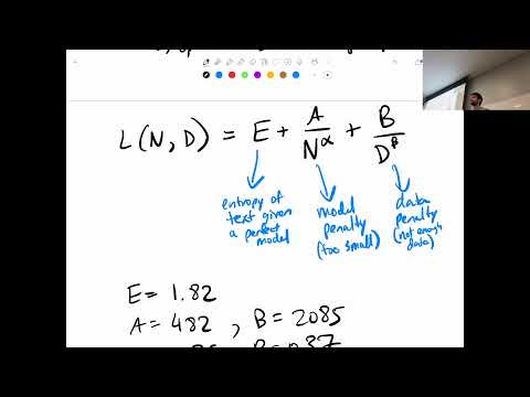
The fitted power law predicts loss from N and D using an irreducible baseline plus a model-size penalty and a data-size penalty.
The constant E represents the estimated entropy floor of text; the discussed replication fit put it at about 1.82.
The model and data penalties shrink as N and D increase; the fitted exponents are positive, while the other coefficients are empirical fit parameters.
The equation explains why neither a tiny model nor a huge model with too little data achieves the best loss under a fixed compute budget.

1:09:03 Inference Economics: Why Production Models May Favor More Data

Compute-optimal training is not always the production objective: inference cost depends strongly on the model served, not on how many tokens it saw during training.
For services with billions of users, a smaller model can reduce repeated inference FLOPs, even if training it on more data costs more upfront.
Mixture-of-experts models can reduce active parameters per inference by routing inputs to only part of the full model.
A company may therefore accept higher one-time training expense to serve a cheaper, smaller model at scale.

Summary, takeaways, and chapters were generated by AI from the video's transcript and may contain errors. The video belongs to its creator, Mohit Iyyer.