Princeton Intro to Robotics (Fall 2026) | Lecture 2: Discrete Motion Planning
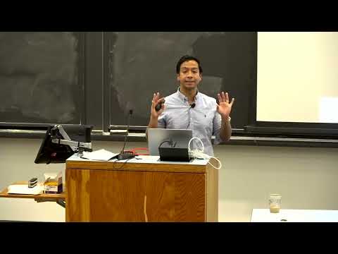 Watch on YouTube →
Overview
Geometric motion planning finds a collision-free path between configurations in a known environment, initially assuming the robot can execute any continuous path and knows its state perfectly. The lecture formalizes configuration space and collision-free space, then discretizes a point-robot environment into a graph and compares breadth-first search with A*, whose admissible cost-to-go heuristic can guide search while preserving optimality.
Key takeaways
- Configuration space turns robot geometry into a planning space: for a planar quadrotor, SE(2) combines x and y position with orientation, and collision states form C_obs.
- Grid discretization creates a graph by mapping free cells to vertices and allowable moves to edges; resolution and four- versus eight-connectivity affect both route availability and search cost.
- BFS guarantees a minimum-hop route on an unweighted graph because it explores paths in increasing order of hop count, but it does not optimize unequal energy or motion costs.
- A* ranks states by f(x) = c(x) + h(x); an admissible heuristic such as Manhattan distance on a four-connected grid can reduce search while preserving optimality.
- Dijkstra's algorithm is the A* special case with h(x) = 0, while negative edge costs invalidate the ordinary shortest-path setup because repeated cycles can drive total cost toward negative infinity.
- Heuristic quality strongly affects practical search effort: the Tesla AI Day example cited approximately 400,000 expanded nodes for a weak Euclidean heuristic versus 22,000 with a navigation-route heuristic.
Chapters
0:00
Course Roadmap: From Drone Navigation to Planning and Learning
- A final-project drone uses an IMU, optical-flow camera, and forward-facing camera to avoid randomly placed obstacles and locate a book.
- The course progresses through planning and control, localization and mapping, and robot learning, including imitation and reinforcement learning.
- Initial planning assumes the environment geometry is already represented, setting up later relaxation of mapping and state-estimation assumptions.
3:00
Geometric Planning and the Piano Movers Problem
- Geometric motion planning searches for a collision-free route between a robot's starting and goal configurations in a known map.
- The piano movers problem illustrates the difficulty of accounting for both a robot's shape and complex environment geometry.
- The general problem is described as PSPACE-complete, reflecting its computational difficulty.
6:03
Motion Planning Applications: Zoox, Protein Folding, and Rubik's Cube
- A Zoox autonomous-vehicle visualization shows a changing geometric map and an updated green path as pedestrians and cars move.
- Autonomous vehicles can incorporate scene semantics, such as whether a nearby pedestrian appears distracted by a phone.
- Protein folding has been approached as planning between molecular configurations, while AlphaFold represents a later deep-learning-based approach.
- Rubik's Cube solving is discrete planning: search among a finite set of cube states for any configuration with matching face colors.
10:04
Planning Assumptions: Feasible Paths, Known State, and Known Map
- The geometric-planning setup treats any continuous path between configurations as executable, even though a car cannot move directly sideways.
- The robot is assumed to know its state perfectly and to follow the planned path without error.
- The environment map is provided in advance; later course material will relax these assumptions through dynamics and localization.
12:00
Degrees of Freedom in Pendulums, Drones, and Snake Robots
- Degrees of freedom count independent motions, or equivalently the minimum number of coordinates needed to specify a configuration.
- A planar pendulum has one degree of freedom, its angle; a planar quadrotor has three, x, y, and orientation θ.
- A planar snake robot with n links and a movable base has n + 2 degrees of freedom: two base-position coordinates and n link angles.
- A pendulum's x and y coordinates are constrained by its fixed length, so they are not independent.
21:44
Configuration Space and Collision-Free Configurations
- Configuration space C is the set of all possible system configurations; a point in C identifies one complete robot pose.
- A point in D dimensions has configuration space R^D, a planar pendulum has S¹, and a planar quadrotor has SE(2), equivalent to R² × S¹.
- A planar n-link snake has configuration space R² × (S¹)^n, capturing base position and each link orientation.
- C_free contains configurations with no collision, while C_obs is its complement in C.
27:35
Visualizing Configuration-Space Obstacles in Three Dimensions
- A triangle robot moving in a plane has a three-dimensional configuration space: x, y, and orientation.
- The orientation dimension wraps around because 0 and 2π represent the same pose.
- Each point inside a configuration-space obstacle corresponds to a triangle pose that collides with an environment obstacle.
- A geometric planning solution is a continuous path in C_free from initial configuration Q_A to goal configuration Q_B.
33:10
Discretizing Continuous Space into a Grid
- The lecture models the robot as a point in a two-dimensional space and overlays a grid to create a finite planning problem.
- Uniform grid cells are a simplifying choice; adaptive resolution could use finer cells near obstacles and narrow passages.
- Four-connectivity permits north, south, east, and west moves, while eight-connectivity also permits diagonals.
- Finer grids can reveal narrow routes but increase the number of states and computational effort.
37:07
Building a Search Graph from Free Grid Cells
- Each grid cell becomes a graph vertex, conventionally placed at the cell center rather than at a corner.
- Edges connect neighboring cells according to the chosen movement rule, such as four- or eight-connectivity.
- Vertices whose cells intersect obstacles, along with their incident edges, are removed.
- The resulting graph converts collision-free grid motion into a standard graph-search problem.
40:09
Breadth-First Search: Queue Expansion and Visited States
- The example searches a grid from configuration (2, 3) to (5, 5), storing frontier vertices in a first-in, first-out queue.
- BFS removes the earliest queued vertex, checks its neighbors, and marks newly discovered cells visited before adding them to the queue.
- A fixed neighbor-order convention determines which equally distant route is explored first.
- Visited-state tracking prevents the search from repeatedly adding cells reached through different paths.
47:41
Recovering Paths and Contrasting BFS with DFS
- To reconstruct the route, record each discovered vertex's parent and backtrack from the goal to the start.
- BFS uses first-in, first-out queue ordering; depth-first search can use a last-in, first-out stack to follow one branch before backtracking.
- BFS finds a minimum-hop path because it explores paths of length k before paths of length k + 1.
- Minimum-hop optimality does not guarantee minimum energy or travel cost when edge costs differ.
50:30
Why A* Improves on BFS and How Path Costs Are Defined
- BFS can expand broadly in every direction and only optimizes hop count, motivating A*'s goal-directed search and support for varied costs.
- A plan's total cost is the sum of its edge costs; costs must be nonnegative to avoid endlessly reducing path cost by cycling over a negative edge.
- A* prioritizes vertices using f(x) = c(x) + h(x), where c estimates cost from the start and h estimates remaining cost to the goal.
- For the presented A* variant to guarantee an optimal path, h must be an underestimate of the true optimal cost-to-go.
1:00:23
A* Heuristics, Manhattan Distance, and Dijkstra's Algorithm
- Manhattan distance is an inexpensive admissible heuristic on a four-connected grid: count horizontal and vertical steps while ignoring obstacles.
- Ignoring obstacles gives a lower bound because actual routes may need extra steps to go around them.
- Setting h(x) = 0 for every vertex reduces A* to Dijkstra's algorithm, which expands by accumulated cost.
- A* combines cost already incurred with estimated remaining cost, directing expansion toward promising routes without abandoning its optimality guarantee when h is admissible.
1:10:29
A* Grid Walkthrough and Learned Heuristics in Vehicle Planning
- The grid example computes c, h, and f for each frontier cell; from the start, c is zero and the Manhattan estimate to the goal is five.
- A* selects the frontier vertex with the lowest f value, using a tie-breaking rule when multiple vertices share that priority.
- A heuristic can be misled by obstacles or adversarial layouts, but useful estimates often reduce exploration compared with BFS.
- A Tesla AI Day example contrasts a weak Euclidean-distance heuristic, which expanded about 400,000 nodes, with a navigation-route heuristic that reduced the search to about 22,000 nodes.
- Learned heuristics and continuous optimization can further guide vehicle planning toward trajectories that account for costs such as passenger comfort.
Summary, takeaways, and chapters were generated by AI from the video's transcript and may contain errors. The video belongs to its creator, Introduction to Robotics @ Princeton.