ME2120 - Dynamics

Overview

Professor Ryan C. Cooper uses a spring-mass accelerometer to connect measured voltage signals with predicted motion, showing how dynamics can help calibrate sensor output into displacement. The class interprets phase-shifted X and Y signals as an elliptical path, relates an impulse of 5 mN·s to initial momentum, and reviews a reusable dynamics workflow: identify degrees of freedom, define kinematics, then apply kinetics.

Key takeaways

An accelerometer's spring-mass response must be modeled dynamically because the mass continues moving after an impulse; voltage readings alone do not directly specify displacement.
When X and Y signals oscillate at the same frequency but have a phase offset, plotting them against each other produces an ellipse rather than a straight-line path.
A measured voltage-to-displacement relationship can be calibrated empirically, then compared with the mass-spring model's predicted motion.
Impulse is directional: a 5 mN·s impulse along negative Y produces an initial momentum change in that direction, with initial velocity found by dividing by mass.
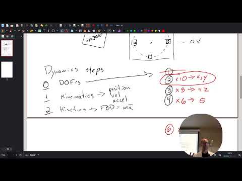
A reusable dynamics method is to identify degrees of freedom, define position and its derivatives through kinematics, then apply force equations through kinetics.
The accelerometer can be modeled with two translational degrees of freedom in its plane; a freely moving rigid body in three dimensions may require six coordinates when orientation matters.

Chapters

0:00 Spring-Mass Accelerometers and Dynamic Response

Cooper models an accelerometer as a mass attached to a spring, often microfabricated from silicon.
Displacement changes the spring force, allowing acceleration to be inferred through the mass-spring relationship.
Predicting the sensor's motion after an impulse is necessary to interpret its measured response.

3:00 Reading X and Y Voltage Signals as Motion Data

The X and Y voltage traces oscillate around an assumed zero-voltage center.
Voltage is not position by itself; calibration is needed to map a voltage change to a displacement such as 10 millimeters.
The recurring reversals in the traces indicate that the mass is moving back and forth.

10:00 Using Phase Differences to Infer an Elliptical Path

Cooper compares paired X and Y voltage values to plot points in a two-dimensional position plane.
The two signals reach their peaks at different times, so the mass does not travel along a fixed diagonal.
Same-frequency sine-like signals with a phase offset produce a circular or elliptical path, with unequal signal magnitudes scaling the axes.

15:00 Matching Predicted Motion to Accelerometer Measurements

The mass-spring model can predict the sensor's motion and an ideal, noise-free version of its X-Y trajectory.
Comparing the predicted ellipse with measured voltage data helps determine how voltage maps to displacement.
Cooper notes that a linear calibration can be measured empirically rather than derived entirely from first principles.

20:00 Planning the Dynamics Solution and Identifying Impulse

Cooper gives the class an open-ended problem-solving period to decide how to start analyzing the sensor motion.
The discussion identifies impulse as a useful way to describe the initial impact that sets the mass moving.
The impulse example connects force applied over a short time with the object's change in momentum.

30:00 Applying a 5 mN·s Impulse to Find Initial Velocity

Impulse is a vector because force has direction, while the time interval is a scalar.
For the impact along negative Y, the impulse is 5 mN·s in the negative-Y direction.
Using impulse-momentum, the initial Y momentum is mass times initial Y velocity, so the impulse determines the mass's initial velocity component.

36:00 Capacitive Displacement Sensing and Measurement Forces

Capacitive displacement sensors register position changes through changing capacitance rather than necessarily applying a significant force.
Cooper distinguishes sensing effects from forces that meaningfully alter the motion in the spring-mass model.
He notes that electrostatic effects could matter for very small masses and weak springs, but are negligible for the larger-scale example.

38:00 The Three-Step Dynamics Workflow: DOF, Kinematics, Kinetics

Step 0 is to identify the system's degrees of freedom before writing equations.
Step 1 defines position, velocity, and acceleration through kinematics.
Step 2 uses a free-body diagram and Newton's second law, with force equal to mass times acceleration, to model kinetics.

43:00 Defining Degrees of Freedom for the Moving Mass

A degree of freedom is an independent quantity needed to specify a system's state or location.
For a point-like mass moving in a plane, X and Y position give two degrees of freedom.
Adding Z position describes translation in three dimensions, while velocity is determined from position over time rather than automatically counting as another independent degree of freedom.

47:00 Choosing a Two-Coordinate Model Instead of Six Rigid-Body DOF

A rigid body moving freely in three dimensions can require six degrees of freedom: three position coordinates and three orientation angles.
Cooper recommends starting with two degrees of freedom for the accelerometer example, tracking only X and Y motion.
The simpler model is easier to analyze, while adding rotational coordinates is appropriate only if the system's rotation matters.

Summary, takeaways, and chapters were generated by AI from the video's transcript and may contain errors. The video belongs to its creator, Professor Ryan C. Cooper.