ME2120 - Dynamics

Overview

Ryan C. Cooper uses a four-bar linkage project to show how engineers reverse-engineer mechanisms, troubleshoot their models, and turn motion plots into useful quantities. Examples include estimating a Texas pump jack’s geometry and oil-pumping stroke, relating crank speed to windshield-wiper motion, and modeling knee ligaments while diagnosing solver branch changes and kinematic locking.

Key takeaways

A four-bar model should be judged by the outputs relevant to its application: windshield-wiper rocker angle and speed, pump-jack stroke and cycle rate, or knee-bone path and range of motion.
Changing a crank’s angular speed from 10 to 100 radians per second does not make a design more realistic; with a roughly 1-meter wiper, 100 radians per second implies about 100 meters per second of tip speed.
A rough pump-jack model can be built from a visual scale estimate: Cooper uses an approximately 15-foot structure and links near 3, 7, and 9 feet, then relates rocker angular travel to stroke length.
Four-bar solvers can converge to different valid geometric configurations; initial guesses and input ranges help select the intended branch and avoid apparent kinematic locking.
For the simplified knee linkage, useful validation targets include the femur’s motion trace and theta 2 range, while realistic knee flexion requires restricting the input instead of allowing a full 360-degree rotation.

Chapters

0:00 Project 2: Design and Quantify a Four-Bar Linkage

Project 2 focuses on designing or reverse-engineering a four-bar linkage and explaining what it does, how it was modeled, and why that design was chosen.
Cooper emphasizes that graphs are tools for examining engineering numbers, not merely attractive pictures.
The class begins with code troubleshooting and encourages deliberately testing model limits by finding cases where outputs fail.

3:24 Crank Speed, Rocker Motion, and Windshield-Wiper Output

The default crank speed is 10 radians per second; increasing it to 100 changes the speed scale while leaving the linkage’s basic motion pattern intact.
For a windshield wiper, the useful output is the rocker-arm angle, such as theta 3, and the resulting wiper speed—not the crank speed alone.
A roughly 1-meter wiper moving at 100 radians per second would imply an implausible speed near 100 meters per second, illustrating why realistic inputs matter.

8:08 Troubleshooting Linkage Models and Testing Design Ideas

Cooper shifts the discussion toward diagnosing Python-model behavior, including outputs and graphs that do not match expectations.
Students explore possible mechanisms such as pump jacks and inverted or differently scaled wiper systems, using the model to test geometry choices.
The troubleshooting approach is iterative: identify what looks wrong, inspect the inputs, and adjust the design rather than assuming the first setup is correct.

16:18 Reverse-Engineering a Pump Jack’s Four-Bar Geometry

A pump jack lifts underground oil by repeatedly moving a large rocker arm up and down; its mass helps the operating mechanism maintain momentum.
Cooper identifies the rocker as link L3, the rotating crank as L1, and the connecting arm as L2.
Using an estimated 15-foot overall scale, he sketches approximate link lengths of 7 feet, 9 feet, and 3 feet, with anchor offsets around dx = -3 feet and dy = 10 feet.
The approximate model runs, demonstrating how observed equipment can be translated into a linkage diagram and tested.

23:28 Pump-Jack Stroke Length and Oil-Pumping Rate

The pump’s practical outputs are how frequently it cycles and how much vertical stroke it produces, since each piston stroke moves a volume of oil.
The rocker’s angular range—approximately 15 degrees to -40 degrees in the example—can be converted to radians and multiplied by the arm length to estimate arc travel.
A longer stroke and more frequent cycles can increase the amount pumped; the model provides quantities that can guide design comparisons.

30:24 Using Negative Link Lengths to Reorient a Mechanism

A student asks whether an inverted windshield-wiper design can be represented with a negative link length.
Cooper explains that the constraint equations can still produce a solution because the sign effectively shifts the angle representation by 180 degrees.
The model may work with this convention, but designers should interpret the resulting angles as reoriented rather than physically negative lengths.

32:16 Building a Knee-Ligament Linkage from MRI Geometry

Cooper sketches a simplified knee mechanism using the patella, tibia, femur, ACL, and PCL, treating the tibia as fixed for a sitting-motion model.
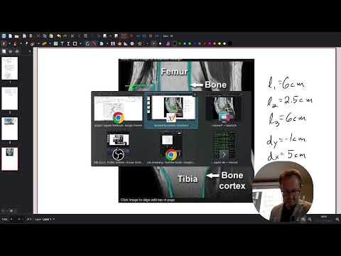
He estimates dimensions from an MRI image, using a 5-centimeter patella as a scale reference and rough linkage lengths around 6, 2.5, and 6 centimeters.
Unlike a crank mechanism, the knee linkage is meant to control bone paths and provide support rather than rotate continuously through 360 degrees.
An initial 0-to-360-degree input is inappropriate for knee motion, so the model is revised to test a more limited angular range.

40:10 Solver Branch Changes and Kinematic Locking in the Knee Model

The knee model initially follows the wrong geometric solution branch; Cooper identifies this as a kinematic-locking or configuration-selection problem.
He adjusts the solver’s initial guesses, including theta 2 and the PCL angle, to steer calculations toward the intended linkage configuration.
Changing the input range and refining geometry improves the motion trace, though the MRI-based dimensions and usable range still need adjustment.
The model’s key outputs are the femur’s traced path and theta 2’s range of motion; Cooper notes that 90 degrees is a useful reference and greater flexion enables deeper squatting.

47:04 Knee-Linkage Interpretation and the Next Dynamics Module

The closing discussion considers how ACL and PCL motion depends on which side of the joint is treated as fixed in the simplified model.
Cooper highlights the geometric significance of the bone’s midpoint and attachment locations in shaping the observed motion.
The next module returns to dynamics: drawing free-body diagrams, forming equations of motion, and solving them using different methods.

Summary, takeaways, and chapters were generated by AI from the video's transcript and may contain errors. The video belongs to its creator, Professor Ryan C. Cooper.