ME2120 - Dynamics

Overview

Professor Ryan C. Cooper uses a NanoHub Jupyter notebook and a four-bar linkage to teach how kinematic constraints predict link positions, paths, and speeds. The analysis uses a prescribed crank rotation to solve for the connector and rocker motions, while emphasizing that geometry-only kinematics does not determine forces or power.

Key takeaways

A four-bar linkage has three moving links and a fixed ground link; prescribing the crank angle lets two constraint equations determine the connector and rocker angles.
The notebook models kinematics—geometry and motion—not the forces or power required to produce that motion.
At 10 rad/s, a 0.25 m crank moves its endpoint at 2.5 m/s; linear speed requires both angular speed and a distance from the rotation axis.
A connector point can trace a noncircular path even when its endpoints move on circles, enabling mechanisms such as Watt-linkage suspension.
Changing all six geometry and drive inputs at once makes analysis difficult; isolating a ratio such as crank length to connector length produces clearer design insight.
Jagged motion plots and a moving trace for fixed hinge C are practical warnings of solver branch changes, invalid geometry, or operation outside the linkage’s feasible range.

Chapters

0:00 NanoHub Jupyter Setup and Submitting Notebook Work

Launch a personal JupyterHub notebook through the rocket link on the course website after creating a NanoHub account.
Notebook cells contain Markdown or code; click a cell to edit it and use Shift+Enter to run or render it.
Submit work as a PDF using File → Print Preview because notebook files and links do not display reliably in HuskyCT.

6:09 Four-Bar Linkage: Three Moving Links and a Fixed Ground Link

A four-bar linkage has four connections but typically three moving parts; the fourth bar is the fixed ground connection between pivots.
A three-bar triangle is kinematically locked when its links are rigid, while a four-bar linkage is the simplest hinged arrangement that can move.
The crank rotates in a circle, the rocker swings back and forth, and the connector joins them; a bicycle crank and windshield wiper illustrate the roles.

13:00 Constraint Equations and Solving the Example Geometry

Two kinematic constraint equations let the model solve for connector angle θ₂ and rocker angle θ₃ when crank angle θ₁ is prescribed.
The sample geometry uses a 0.25 m crank, 1 m connector, 1 m rocker, and fixed-pivot offsets dx = 0.95 m and dy = 0.
The notebook’s prebuilt nonlinear solver can converge to equivalent angles separated by full revolutions, so an appropriate initial guess helps avoid very large reported angles.

18:00 Reading Link Angles and Checking Positions

Angles are measured from the positive x-axis: 0° points right, 90° points up, and 180° points left.
Plots of θ₂ and θ₃ against θ₁ show how the connector and rocker orient as the crank completes a cycle.
Because 0° and 360° represent the same orientation, matching cycle endpoints indicate the mechanism returns to its starting configuration.

22:15 Tracing Crank, Rocker, and Connector Paths

The crank endpoint follows a circle because the model prescribes continuous circular crank motion.
The rocker endpoint traces a back-and-forth path, the same basic motion used to sweep a windshield wiper.
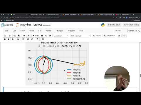
The connector’s midpoint can trace a noncircular curve because its ends are constrained to move on different circles; a Watt linkage can use related geometry to approximate vertical suspension travel.

25:38 Converting Angular Speed into Linear Speed

The example drives the crank at 10 rad/s, about 1.6 revolutions per second, and the connector and rocker angular rates vary through the cycle.
Angular speed alone is not linear speed: multiply angular speed by radius to get tangential speed.
For a 0.25 m crank at 10 rad/s, point A travels at 2.5 m/s; a longer link can produce a higher point speed even while rotating more slowly.

32:00 Choosing a Four-Bar Project and Real-World Applications

Project options include designing a windshield wiper, reverse-engineering a mechanism, or exploring how one geometric ratio affects motion.
Changing all six inputs—L₁, L₂, L₃, dx, dy, and drive rate—creates an unwieldy design-of-experiments problem; varying one relationship at a time is more manageable.
Examples include Watt-linkage suspension and the knee, where the ACL, PCL, and femur geometry contribute to constrained motion; a car piston is instead a slider-crank mechanism.

38:00 Stepping Through Linkage Configurations and Animating a Heart Path

Changing the notebook’s index variable I selects successive configurations, producing static snapshots rather than a continuously running animation.
The notebook can also animate a four-bar geometry; a prepared Valentine’s linkage traces a heart-shaped path.
Geometry changes can disrupt a prepared example, so restoring its original dimensions may be necessary to recover the intended animation.

42:00 Diagnosing Invalid Geometry and Motion Range

Sharp jumps or jagged angle plots signal that the mechanism is not moving smoothly or the solver has switched between solution branches.
A very short connector paired with a long rocker can create an impossible or highly restricted configuration, allowing motion only over a narrow crank-angle range.
The fixed hinge C should remain stationary; a visible yellow trace indicates a violated constraint or geometry outside the valid range.
Crossing lines in a 2D diagram do not necessarily mean physical collision because the links may be arranged in different planes.

Summary, takeaways, and chapters were generated by AI from the video's transcript and may contain errors. The video belongs to its creator, Professor Ryan C. Cooper.