Mathematical Foundations of AI Alignment, Lecture 7 (Calibration as Decision Alignment)

Overview

Aaron Roth frames probability forecasts as a decision interface: users should be able to treat forecasts as correct, choose actions that maximize expected utility, and avoid substantial regret. He shows that calibration bounds the gains from any alternative forecast-to-action rule for every utility function, then introduces decision calibration, which groups forecasts by the action they induce and can provide swap-regret guarantees with only one bias bucket per action.

Key takeaways

Calibration bounds the utility gain from any alternative forecast-to-action rule by a term proportional to the sum of forecast-specific bias norms, making best-response use safe across utility functions.
Overall unbiasedness is insufficient for decision quality: forecasts that are 99% wrong in opposite directions can average out statistically while inducing the wrong action on every case.
Decision calibration controls accumulated bias by induced action rather than exact forecast; with K actions, it requires only K buckets even when the outcome dimension D is large.
A constant forecast equal to the base rate can be calibrated yet uninformative, as shown by the 50%-safe example where users audit every proposal and earn 1/2 per case.
Decision calibration yields a swap-regret guarantee for a specified user's utility function, while full calibration offers a broader utility-agnostic guarantee for many users.
Blackwell approachability is the planned algorithmic tool for obtaining calibration guarantees under arbitrary sequences and distribution shift, including simultaneous guarantees for multiple decision makers.

Chapters

0:00 Forecasts as Interfaces Between AI Predictions and User Decisions

Aaron Roth shifts from eliciting preferences to evaluating forecasts that inform real-world actions.
Users gain utility from downstream decisions and states of the world, not necessarily from an LLM's text itself.
A single forecasting system should support users with different utility functions and decision problems.

4:40 Why Perfect Probabilistic Predictions Are an Unrealistic Standard

A perfect forecast of the underlying state distribution would support every downstream decision maker.
Perfect probabilistic forecasting is too demanding as a practical guarantee.
The desired interface lets users act as if forecasts are correct, even when the guarantee is weaker than perfect prediction.

7:30 Modeling States, Forecasts, Actions, and Expected Utility

The decision-relevant state has D possible outcomes, represented by a probability vector.
A user's utility for each action is a vector with one value per outcome.
Expected utility under forecast P is the inner product of the action's utility vector and P.
A best response selects the action with the highest expected utility under the forecast.

11:00 Safe-System Deployment: A Three-Action Decision Example

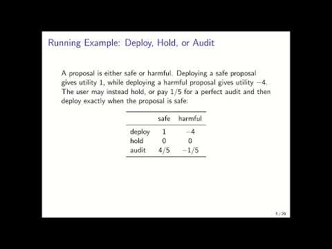
A system can be safe or harmful; deploying it yields 1 if safe and -4 if harmful.
Holding the system yields 0 in either state, while an audit costs 1 and reveals the state.
After auditing, the decision maker deploys only if the system is safe, earning 4/5 after the audit cost.

13:00 Best Responses Divide Safety Forecasts into Decision Regions

For a binary safety outcome, a forecast is summarized by R, the predicted probability that the system is safe.
Expected utilities for deploying, holding, and auditing can each be calculated from R.
The best-response rule partitions forecast probabilities into regions where holding, auditing, or deploying is optimal.

15:00 Decision-Relevant Errors Depend on Action Boundaries

Changing a safety forecast from 0.3 to 0.5 may have no effect if both values lead to auditing.
A smaller shift from 0.19 to 0.21 can matter more if it crosses a best-response boundary and changes the action.
Without knowing a user's utility function, a forecaster cannot know which prediction regions are decision-critical.

21:00 Why Aggregate Unbiasedness Can Still Cause Bad Decisions

In the example, harmful systems are forecast as 99% safe and safe systems as 99% harmful.
The forecast is unbiased overall when safe and harmful systems each occur half the time.
Opposing errors cancel in aggregate, but each forecast still induces the wrong action, so aggregate unbiasedness alone is insufficient.

25:00 Defining Calibration for Sequences Without a Fixed Distribution

Roth models predictions and realized outcomes as a sequence, allowing outcomes to shift over time rather than assuming an i.i.d. source.
For each forecast P, calibration compares P with the empirical outcome frequencies on rounds when P was issued.
In a rain example, a 70% forecast should correspond to rain on roughly 70% of its forecasted days.

33:30 Measuring Calibration Error with Conditional Bias

The unnormalized bias for forecast P is the sum of outcome vectors minus P across all rounds that used P.
Calibration error sums the L1 norms of these forecast-specific bias vectors.
Exact zero bias is generally impossible with finite data: even a correct 50% coin forecast may not match observed frequencies.

36:00 Calibration Bounds Regret from Reinterpreting Forecasts

A reinterpretation rule maps forecasts to actions differently from the user's best response to each forecast.
Regret measures the realized utility gain such a rule would have achieved over best-responding.
The regret decomposition separates utility in a hypothetical world where forecasts are correct from a correction term caused by forecast bias.
Best response is optimal in the hypothetical world, so only the calibration-bias term can create positive regret.

44:30 Calibration Gives a Utility-Agnostic Decision Guarantee

The regret correction is bounded using the maximum L-infinity difference between action utility vectors and the L1 calibration error.
If utilities are normalized to [0,1], the utility-difference constant is at most 1.
Because calibration does not depend on a particular utility function, its decision guarantee holds simultaneously for different downstream users.

46:30 Constant Forecasts Are Calibrated but Can Hide Useful Information

A constant forecast equal to the overall outcome frequency is calibrated because its only calibration condition is aggregate unbiasedness.
In the safe-system example with half safe and half harmful proposals, always predicting 50% safety leads users to audit every proposal.
That policy earns 1/2 per proposal in the example, even if additional information could support better forecasts and decisions.

52:00 Decision Calibration Groups Forecasts by the User's Action

Full calibration controls bias separately for every distinct forecast value, including distinctions irrelevant to a user's action.
Decision calibration instead groups together all forecasts that induce the same best-response action.
With K available actions, decision calibration needs only K bias buckets, rather than a number of forecast buckets that can grow exponentially with outcome dimension D.

59:30 Decision Calibration Allows Biases to Cancel Within Action Buckets

The bias of an action bucket is the sum of outcome-minus-forecast vectors across rounds that induced that action.
Full calibration implies decision calibration because action buckets combine forecast-specific buckets.
Decision calibration is weaker because it controls the norm of the summed biases, allowing opposing forecast errors within an action bucket to cancel.

1:04:30 Swap Regret Tests Whether Best-Response Actions Could Be Remapped

Swap regret compares a user's best-response actions with any hindsight rule that remaps each action to another action.
A remapping can ask, for example, whether every round spent auditing would have been better spent deploying.
Swap regret is stronger than external regret: remapping every action to one fixed action includes the fixed-action comparison, while other remappings allow more nuanced comparisons.

1:08:00 Decision Calibration Controls Swap Regret

The swap-regret proof decomposes realized utility into a forecast-correct term and an outcome-minus-forecast bias term.
Best responding makes the forecast-correct term nonpositive, because the chosen action maximizes expected utility under the forecast.
Within each action bucket, both the best-response action and its remapped comparator are fixed, so their utility-vector difference can be paired with the bucket's accumulated bias.
Cauchy-Schwarz bounds the bias contribution using the L2 norm of each action-bucket bias, yielding a swap-regret bound proportional to decision-calibration error.

1:14:00 The Tradeoff: Personalized Decision Guarantees Versus Universal Calibration

Decision calibration can be easier to obtain in high dimensions because it controls one bucket per action.
Its guarantee is defined relative to a particular user's utility function and action set.
Full calibration's key advantage is that its condition is utility-agnostic and can support guarantees for many different downstream decision makers.

1:20:00 Blackwell Approachability for Adversarial Calibration

Roth previews Blackwell approachability as a way to guarantee calibration properties without assuming a fixed outcome distribution.
The intended algorithms can handle dynamically changing or adversarial outcomes and target decision calibration for multiple utility functions.
Because the forecast determines its own calibration bucket, the algorithm must account for the self-referential link between choosing a forecast and choosing which bias to control.

Summary, takeaways, and chapters were generated by AI from the video's transcript and may contain errors. The video belongs to its creator, Aaron Roth.