Lecture 7c

Overview

The lecture derives backpropagation for a two-layer multilayer perceptron, beginning with scalar computations and extending to mini-batches, vectors, and matrices. It explains how mini-batch SGD approximates the full-data gradient, then uses computation graphs and the chain rule to calculate gradients for weights and biases; cross-validation is distinguished from training as a way to compare hyperparameter choices.

Key takeaways

Mini-batch SGD replaces a full-dataset gradient with an unbiased estimate from B samples; shuffling and processing T batches completes one epoch.
Backpropagation is a computation-graph traversal: calculate intermediate values in a forward pass, then propagate derivatives backward while reusing stored values.
The multivariable chain rule is needed whenever a variable influences the loss through multiple paths, and its gradient contributions must be summed.
Shared weights and biases connect to every example in a mini-batch, so their gradients sum across samples even when sample-specific forward computations are independent.
In matrix-vector layers, one weight-matrix element influences a specific activation or score coordinate, while a hidden activation coordinate may influence several output coordinates; the relevant gradients sum over those connected paths.
Training fits parameters for a fixed model, whereas cross-validation compares separately trained choices such as hidden-node counts or SGD step sizes.

Chapters

0:00 Two-Layer MLP Structure and the Parameters to Learn

The model applies a linear stage, an elementwise hidden activation, and a second linear stage, with an optional output nonlinearity.
Training learns the layer weights and biases; inputs and activation functions are fixed.
The objective averages per-sample losses, typically negative log likelihood, over the training set.

3:00 Mini-Batch SGD Avoids Full-Dataset Gradient Computations

A full gradient update requires processing every training sample, which is impractical for datasets with millions or billions of examples.
Mini-batch SGD estimates the gradient using a subset of size B, then updates parameters with a step size times that estimate.
The training data is shuffled and split into non-overlapping mini-batches; processing all T batches is one epoch, followed by another shuffle.
The mini-batch gradient is unbiased, and reducing the step size reduces its noise but generally requires more updates.

8:00 Computation Graphs Organize Forward and Backward Passes

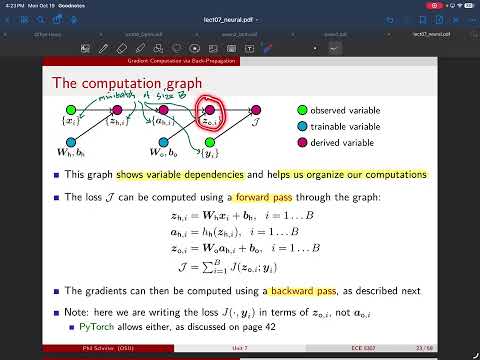
The gradients are needed for hidden weights WH, hidden biases BH, output weights WO, and output biases BO.
A computation graph records dependencies, such as network outputs and labels feeding the loss.
The forward pass computes activations and loss from the current data and parameters; the backward pass moves from loss to parameter gradients.
After the gradients are computed, one SGD update produces new parameters and the next iteration repeats the two passes.

12:00 Forward-Pass Equations and Training Versus Cross-Validation

The forward pass evaluates hidden pre-activations ZH, hidden activations AH, and output scores ZO for each mini-batch item.
The derivation stops at linear output scores ZO, so the loss is written directly in terms of ZO rather than optional soft outputs.
A two-layer network is used to introduce the main gradient ideas before generalizing to multiple hidden layers.
Training minimizes loss for a chosen architecture; cross-validation compares separately trained models or settings such as hidden-node count and learning rate.

16:00 Chain Rule and the Scalar, Single-Sample Computation Graph

For a dependency chain X to Y to Z, the derivative is dZ/dX = (dZ/dY)(dY/dX); already-computed intermediate gradients can be reused.
When X affects Z through multiple intermediate variables, the multivariable chain rule sums the contributions from each path.
The derivation first assumes scalar variables and batch size one, reducing the network to two affine transforms, a hidden activation, and a scalar loss.

22:00 Scalar Backpropagation Through the Output and Hidden Layers

Backpropagation starts with dJ/dZO, computed as the loss derivative evaluated at the forward-pass score ZO.
The output-layer gradient propagates as dJ/dAH = (dJ/dZO)WO, then through the hidden activation using its derivative evaluated at ZH.
The scalar parameter gradients are dJ/dBO = dJ/dZO, dJ/dWO = (dJ/dZO)AH, dJ/dBH = dJ/dZH, and dJ/dWH = (dJ/dZH)X.
Forward-pass values such as X, AH, ZH, and ZO are reused during the backward pass.

30:00 Scalar Network Gradients with a Mini-Batch

With B samples, each sample has its own ZH, AH, and ZO, while all samples share the same weights and biases.
The batch loss sums the individual losses, so the derivative with respect to one ZO element involves only that sample's loss term.
Elementwise activation and affine operations keep different samples decoupled when propagating gradients through ZO, AH, and ZH.
Shared parameters affect every sample, so gradients for BO, WO, BH, and WH sum contributions across the batch.

36:00 Why Shared Parameters Require Summing Across Batch Paths

For a shared output bias BO, the multivariable chain rule sums dJ/dZO_i times dZO_i/dBO over all batch indices i.
For a shared output weight WO, the same batch sum applies, with each derivative dZO_i/dWO equal to AH_i.
Hidden biases and weights also accumulate contributions over the batch; their local derivatives use 1 for BH and X_i for WH.
The key distinction is that sample-specific activations remain independent, while a shared parameter connects to every sample's loss.

42:00 Extending Backpropagation to Vector Activations and Matrix Weights

The full case uses vector-valued features, biases, hidden activations, and targets, plus matrix-valued weights.
Derivatives are computed element by element rather than by treating a whole vector or matrix as a single scalar variable.
For an output score vector, a selected score coordinate contributes its loss derivative for the matching batch item.
A single hidden activation coordinate can affect multiple output coordinates through a column of WO, so its gradient sums across those output-coordinate paths.

48:00 Elementwise Activations and Output-Bias Gradients

The derivative from hidden pre-activation ZH_i,l to activation AH_i,l uses the activation derivative evaluated at ZH_i,l.
Elementwise activations decouple coordinates: changing one ZH coordinate affects only the matching AH coordinate.
An output-bias coordinate BO_k affects the matching output coordinate for every batch item, requiring a sum over batch index i but not over output coordinate k.
The local derivative of output coordinate ZO_i,k with respect to BO_k is 1.

54:00 Matrix-Weight Gradients, Index Checks, and Next Steps

An output-weight element WO_k,l affects output coordinate k through hidden coordinate l, giving a batch sum whose local factor is AH_i,l.
For a hidden-weight element WH_l,j, the local factor is input coordinate X_i,j; summing over batch index i leaves the expected matrix indices l and j.
The index sanity check is to ensure summed indices disappear while the indices of the parameter being differentiated remain.
The lecture closes by previewing vector-and-matrix notation, implementation details, and networks with more than one hidden layer.

Summary, takeaways, and chapters were generated by AI from the video's transcript and may contain errors. The video belongs to its creator, Prof. Schniter.