Lecture 7b

Overview

The lecture develops a two-layer multilayer perceptron (MLP) for nonlinear classification, then generalizes its activation functions and losses to binary classification, multiclass classification, and regression. It explains why neural-network training is non-convex, motivates mini-batch stochastic gradient descent (SGD) as a cheaper unbiased gradient estimate, and introduces epochs and computation graphs as preparation for backpropagation.

Key takeaways

A hidden layer can turn a nonlinearly separable dataset into a linearly separable representation by learning multiple sigmoid features, as in the four-feature example that isolates a trapezoidal region.
Nonlinear hidden activations are essential: composing linear layers without them collapses to a single linear transformation and does not overcome linear separability limits.
Output activations and loss functions must be paired consistently: binary sigmoid outputs use probability-based binary cross-entropy, while raw scores require the corresponding score-based likelihood.
Gaussian observation noise leads to quadratic regression loss, whereas a Laplace noise model leads to absolute-error loss that is less sensitive to outliers.
Uniformly sampled mini-batches yield unbiased estimates of the full training gradient, allowing SGD to reduce per-update computation while introducing zero-mean trajectory noise.
An epoch processes the full training set once through non-overlapping mini-batches, then reshuffles the samples before the next pass.

Chapters

0:00 Learnable Nonlinear Features Solve a Circular Classification Problem

A class arranged in the middle of another class cannot be separated well by a linear decision boundary in the original two features.
Adding a feature such as the sum of the original features squared can make the transformed data linearly separable.
A neural network learns a parameterized feature transformation from training data rather than requiring the transformation to be designed manually.

6:49 A Two-Stage MLP Learns Four Sigmoid Features

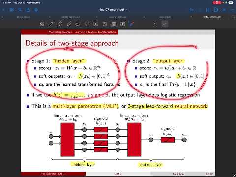
The example uses four hidden units, each applying a logistic sigmoid to a linear score to produce a value between 0 and 1.
The four soft outputs encode regions of the input space; the example’s trapezoid maps approximately to the feature vector 0, 0, 1, 0.
A second linear classifier separates that hidden-feature vector from vectors produced elsewhere, with training based on binary cross-entropy.

10:49 MLP Parameters, Training Loss, and Non-Convex Optimization

The hidden layer applies a linear transformation followed by an elementwise sigmoid; the output layer maps those activations to a final score or probability.
The learnable parameters are the hidden- and output-layer weights and biases; together, the layers form a two-stage feed-forward MLP.
Gradient descent can minimize the binary cross-entropy objective, but hidden-layer nonlinearities make the loss non-convex, so optimization may reach a local minimum or saddle point rather than a global minimum.

12:05 Generalizing MLP Layers and Choosing Hidden Activations

An MLP can have multiple output scores, including one score per class for one-versus-rest classification; hidden activation functions must be nonlinear to add expressive power.
Stacking linear layers without nonlinear activations still produces a linear mapping and therefore cannot solve general nonlinearly separable problems.
The sigmoid is bounded from 0 to 1 but centered at 0.5; a shifted and scaled version is centered at zero and bounded from -1 to 1.
ReLU passes positive inputs unchanged and maps negative inputs to zero; it is unbounded and not zero-centered, but remains a widely used hidden-layer activation.

15:13 Output Activations for Binary and Multiclass Classification

For binary classification, the output can be the raw score z or its logistic sigmoid; predictions can be made by thresholding z at zero.
The loss must match the output representation: use binary cross-entropy for sigmoid probabilities or the corresponding negative log-likelihood written for raw scores.
For K-class classification, the output layer produces K one-versus-rest scores; softmax is the standard probability-producing activation, while raw scores can also be used with a compatible loss.

22:55 Regression Outputs and Likelihood-Based Loss Functions

For regression with K targets, the MLP typically outputs K linear estimates without applying an output activation.
Assuming Gaussian noise around each prediction makes the negative log-likelihood a quadratic loss summed across training examples and target dimensions.
A Laplace-noise assumption instead leads to an absolute-error loss, which can be more suitable when observations contain outliers.

27:52 Why Full-Batch Gradient Descent Becomes Impractical

The training objective averages the per-example losses across all n training samples; its full gradient therefore requires contributions from every sample at each update.
For datasets with millions or billions of examples, repeatedly computing that full gradient is expensive.
On an elongated cost surface, gradient descent can initially move in a direction that is not directly toward the minimum, motivating cheaper approximate updates.

33:04 Mini-Batch SGD Estimates Gradients from Shuffled Samples

SGD shuffles the training data and estimates the gradient using a mini-batch rather than all n examples.
Typical mini-batch sizes cited include 16, 64, and 128 samples; the update averages the per-example gradients within the selected batch.
Different batches produce different gradient estimates, reducing computation per update at the cost of random variation.

36:53 Why Mini-Batch Gradients Are Unbiased—and Noisy

When batch indices are sampled uniformly, each training example has inclusion probability equal to the batch size divided by n, making the mini-batch gradient an unbiased estimate of the full gradient.
SGD updates are therefore correct on average, although individual parameter trajectories fluctuate around the full-gradient path.
The learning rate scales the effect of gradient noise: smaller batches generally require more cautious step sizes, while larger batches can tolerate larger steps.

45:47 Batch Size, Iterations, and Training Epochs

Let B denote the mini-batch size and n the number of training samples; the number of batches per epoch is the ceiling of n divided by B.
Mini-batches are non-overlapping within an epoch, so one SGD iteration per batch processes every training example once.
After the final batch, the data are reshuffled before the next epoch so that the batches contain different sample groupings.

50:09 Backpropagation Begins with a Computation-Graph Forward Pass

Backpropagation is introduced as an organized, computer-executable procedure for calculating gradients through a multilayer network.
A computation graph records direct variable dependencies so that gradient calculations can be organized as a forward pass followed by a backward pass.
The forward pass computes hidden scores from inputs and parameters, hidden activations, output scores, and then a scalar mini-batch loss across B examples.

Summary, takeaways, and chapters were generated by AI from the video's transcript and may contain errors. The video belongs to its creator, Prof. Schniter.