Lecture 7a

Overview

A two-layer feed-forward neural network can classify nonlinearly separable data by learning hidden features: each hidden node applies a nonlinear activation to an affine transform, and an output layer combines those features. The lecture develops this idea from a four-node sigmoid example, explains why hidden-layer nonlinearities matter while an output sigmoid can be optional, and introduces binary cross-entropy, non-convex optimization, network structure, and common activations including sigmoid, tanh, and ReLU.

Key takeaways

A neural network can learn a useful feature map by training hidden-layer affine transforms and nonlinear activations jointly with the output classifier.
Without hidden-layer nonlinearities, any cascade of affine layers collapses to one affine transform, so it cannot solve a problem that requires a nonlinear decision boundary.
For binary classification, the final sigmoid can be omitted when the score itself is used for prediction and the loss is expressed directly in terms of that score; hidden nonlinearities cannot be omitted for the same reason.
Adding hidden units increases representational capacity but can raise overfitting concerns, while the network’s non-convex loss also means gradient descent may converge to different local minima from different initializations.
Sigmoid, tanh, and ReLU have distinct output ranges and optimization behavior; initialization strategies should be matched to the chosen activation rather than treated as interchangeable.

Chapters

0:00 Why Linear Classifiers Fail on Nonlinearly Separable Data

A two-feature classification example places green and blue targets so no single linear decision boundary separates the classes well.
Adding a nonlinear feature such as x₁² + x₂² can make the transformed data linearly separable in three dimensions.
Neural networks address the generic feature-engineering problem by learning useful nonlinear transformations from labeled data.

2:49 Four Sigmoid Classifiers Build Learned Features

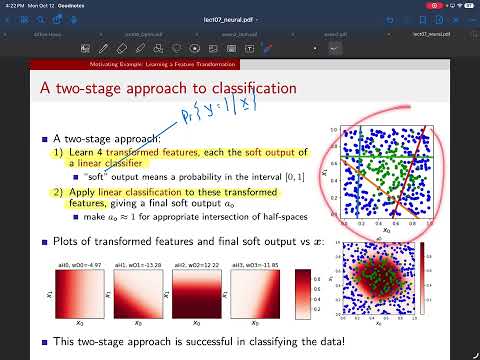
The first stage uses four linear classifiers, each followed by a logistic sigmoid to produce a feature between 0 and 1.
A hidden feature is 0.5 on its classifier’s decision boundary; it approaches 1 or 0 on opposite sides.
The four outputs form a vector that can encode which side of each learned boundary contains an input.
A second linear classifier can recognize a particular hidden-output pattern, such as the pattern associated with the interior target region.

8:20 Reading Hidden-Layer Heat Maps and Output Patterns

Each heat map displays one hidden classifier’s sigmoid output across the two-dimensional input space, with values near 1 on one side and near 0 on the other.
The four first-stage outputs jointly identify regions formed by intersecting half-spaces; one region is illustrated by the approximate pattern 0, 0, 1, 0.
The output-layer weights and bias combine that pattern to produce high final probabilities within the desired region and low probabilities outside it.

16:40 Two-Layer Perceptrons Learn Their Boundaries from Data

The block diagram maps two input features through a matrix of hidden-layer weights and four biases, then applies sigmoid activations.
The output layer combines the four hidden activations with its own weights and bias to produce a classification score.
Training adjusts both layers’ weights and biases using labeled examples, negative log-likelihood, and gradient descent.
The objective is non-convex, so different random initializations or training paths can produce different parameter values and local minima.

22:03 Hidden-Unit Count and the Need for Nonlinear Activations

Two hidden units may be insufficient to represent the illustrated class geometry, while four units can create the needed regions.
Adding many units can raise overfitting concerns under classical statistical learning, although neural-network behavior can be more complicated.
Cascading affine transformations without a nonlinear activation still produces an affine transformation, reducing the network to a linear classifier.
Hidden-layer nonlinearities are therefore essential for representing decision boundaries that a linear classifier cannot express.

25:54 Why the Output Sigmoid Can Be Omitted

For binary classification, the sign of the final linear score can determine the predicted class without converting the score through a sigmoid.
The sigmoid maps a real-valued score to a probability and is invertible, so it does not add information to the score.
The lecture notes that binary cross-entropy can be written directly in terms of the score, making the output sigmoid unnecessary for training as well as prediction in this setup.
The hidden activations remain necessary: unlike the output sigmoid, they provide the nonlinearity that gives the network its added expressive power.

29:50 Binary Cross-Entropy and Non-Convex Network Training

The training set consists of input-feature vectors paired with binary labels, and binary cross-entropy measures the fit of predicted outputs to those labels.
The full network’s processing from raw features to final output is grouped into a parameterized function f.
Hidden-layer nonlinearities make the loss non-convex in the network parameters, unlike standard logistic regression’s convex objective.
Gradient descent may settle at a local minimum; the lecture flags practical optimization techniques as a later topic.

34:17 Biological Neurons and Three Phases of AI

The neuron analogy maps dendrites to inputs, the soma to weighted accumulation, a threshold-like activation to nonlinear processing, and the axon to the output.
The historical overview traces early neuron models in the 1940s and perceptrons in the 1950s, followed by periods of limited progress and renewed interest.
The current deep-learning phase is described as emerging around 2012, when more data and computation enabled breakthroughs in speech and image processing.
Earlier signal-processing methods remained useful when training data and computational resources were insufficient for neural networks to outperform them.

41:10 General Two-Layer Network Dimensions and Activations

For d input features, the hidden layer applies a learned affine transform followed by a scalar activation at each node.
A network can use many hidden nodes; each node typically applies the same activation function independently.
The output layer can produce a vector through a matrix transform and bias vector, followed by an optional vector-valued nonlinearity.
Additional hidden layers repeat the affine-transform-and-activation structure, forming a deeper network.

44:18 How to Read Neural-Network Diagrams

Some computer-science diagrams draw nodes as data and arrows as computation, opposite to the signal-flow convention common in electrical engineering.
In the lecture’s preferred engineering-style diagrams, signals travel along wires and processing occurs inside boxes.
Hidden layers use separate scalar activations, while the output stage may apply one joint multi-input, multi-output transformation.

47:47 Sigmoid, Tanh, and ReLU: Tradeoffs and Initialization

The sigmoid is bounded between 0 and 1 but is not centered at zero; tanh has a similar shape and ranges from −1 to 1.
ReLU outputs max(0, z): it clips negative inputs to zero and passes positive inputs through, and it is commonly used in deep networks.
Activation choice affects optimization and the shape of the loss surface; ReLU is not differentiable at zero, and no activation is best for every dataset.
Weight initialization must suit the activation: the lecture warns that a PyTorch default designed for ReLU may not work well with sigmoid, and vice versa.

Summary, takeaways, and chapters were generated by AI from the video's transcript and may contain errors. The video belongs to its creator, Prof. Schniter.