Lecture 6d

Overview

Gradient descent minimizes a loss by repeatedly stepping opposite its gradient, but its results depend on initialization and learning rate; a finite-difference-style linearization check can catch incorrect gradient code. The lecture connects convergence guarantees to convexity, defines convex sets and functions, and introduces constrained optimization through Lagrange multipliers and KKT conditions.

Key takeaways

Validate a hand-derived and coded gradient by checking whether nearby loss differences match the gradient’s inner product with the parameter displacement; a 1e-6 perturbation balances approximation accuracy and floating-point limitations.
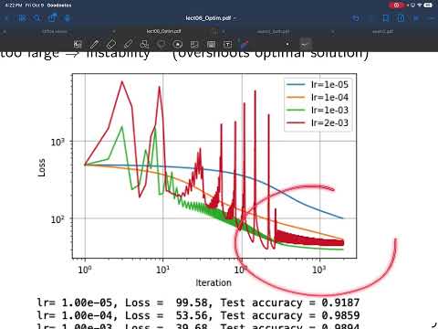
Learning rate controls the speed-versus-stability tradeoff: in the breast cancer example, 1e-4 remained convergent but unfinished after 2,000 iterations, while larger steps overshot or oscillated.
For differentiable convex objectives, a sufficiently small gradient-descent step size and enough iterations can reach a global minimizer; non-convex objectives may instead have multiple local minima.
Convexity can be checked through curvature: scalar functions have nonnegative second derivatives, while vector-input functions require a positive-semidefinite Hessian.
Equality constraints can be incorporated with one Lagrange multiplier per constraint, while inequality constraints require multipliers and KKT conditions to distinguish active from inactive constraints.
Ordinary gradient descent is not a universal optimizer: nonsmooth objectives such as lasso, curvature-aware Newton methods, adaptive step sizes, and momentum call for different techniques.

Chapters

0:00 Gradient Descent Basics and a Numerical Gradient Check

Gradient descent starts from an initialization and repeatedly steps downhill on objective J(W), generally reaching a local minimum determined by the starting point.
The first-order approximation predicts J(W1) − J(W0) using the gradient at W0 dotted with W1 − W0.
Check gradient code by comparing actual and predicted loss changes for nearby random parameter vectors; a perturbation scale of 1e-6 typically gives about five or six matching decimals.
Avoid perturbations smaller than floating-point precision, and precompute reusable quantities such as matrix A during problem initialization.

6:55 Gradient Descent Implementation and Learning-Rate Experiments

The implementation takes a cost-and-gradient function, initial parameters, learning rate, and iteration count; it can save loss and parameter histories for debugging.
On the breast cancer data demo, a standard-normal initialization, 2,000 iterations, and a 1e-4 step size still showed a decreasing loss at the final iteration.
A step size 10 times smaller converged more slowly, while a 10-times-larger step overshot the minimum and caused temporary loss increases.
Increasing the step size by another factor of two caused persistent oscillation; plotting loss and iteration on logarithmic axes makes these trajectories easier to compare.

13:55 Convex Sets: Line Segments Stay Inside

A set is convex when every point on the line segment between any two members remains in the set.
The segment between x and y is expressed as the convex combination t·x + (1−t)·y for 0 ≤ t ≤ 1.
Circles, rectangles, ellipses, hyperplanes, half-spaces, and all of Rⁿ are examples of convex sets; a set with a segment extending outside it is non-convex.

16:15 Convex Functions and Global-Minimum Guarantees

A function is convex when its domain is convex and its value at any convex combination of inputs is no greater than the same combination of its endpoint values.
Linear functions, norms, and sums of convex functions are convex; composing convex functions also preserves convexity when the outer function is nondecreasing.
For scalar inputs, a nonnegative second derivative indicates convexity; for vector inputs, the Hessian must be positive semidefinite.
RSS, binary cross-entropy, cross-entropy, and their L1- or L2-regularized forms are convex examples; a local minimum of a convex function is also global.

23:40 Equality and Inequality Constraints with Multipliers

Constrained optimization minimizes J(W) subject to equalities hₗ(W)=0 and inequalities gₘ(W)≤0.
For equality constraints, form an augmented objective J(W) + Σₗ λₗhₗ(W), assigning one Lagrange multiplier λₗ to each equality.
Stationarity with respect to λₗ imposes hₗ(W)=0, linking the augmented optimization problem to the original equality requirements.
Inequality constraints introduce multipliers μ and require KKT conditions, which account for constraints that are active at the solution versus those that are not.

28:40 Beyond Basic Gradient Descent: SGD, Newton Methods, and Momentum

Later topics include stochastic gradient descent and practical strategies for non-convex optimization, where a global optimum may be difficult to establish.
Adaptive learning-rate methods adjust step sizes during optimization, while Newton’s method uses local curvature and can take fewer but more expensive steps.
Nondifferentiable objectives such as lasso need methods beyond ordinary gradient algorithms; momentum is another practical technique not covered in detail.

Summary, takeaways, and chapters were generated by AI from the video's transcript and may contain errors. The video belongs to its creator, Prof. Schniter.