Lecture 6c

Overview

The lecture develops gradient descent from the geometry of stationary points through a Taylor-series argument for choosing a sufficiently small learning rate. It then derives the multivariable chain rule for binary logistic regression and translates the result into efficient NumPy/Python code, including a class that caches the feature matrix.

Key takeaways

A zero gradient is necessary for an interior differentiable optimum but does not identify its type: stationary points can be minima, maxima, or saddles.
Convexity removes the local-versus-global ambiguity: any local minimum of a convex objective is also a global minimum.
Gradient descent updates parameters by w^(k+1) = w^k − α_k∇J(w^k); a learning rate that is too large can overshoot and increase the objective.
A Taylor expansion explains why sufficiently small positive steps decrease cost: the useful term scales with α, while the bounded higher-order error scales with α².
For binary logistic regression with scores z = Aw, the gradient is Aᵀ(σ(Aw) − y), where σ is the sigmoid function.
Precomputing and caching A in a Python class avoids rebuilding the augmented feature matrix on every gradient-descent iteration.

Chapters

0:00 Gradient Recap: Taylor Approximations and Steepest Ascent

A scalar-output function's gradient collects its partial derivatives; matrix-valued inputs can produce matrix-shaped derivatives.
A first-order Taylor approximation uses the function value and gradient, with higher-order error represented by a big-O term proportional to squared distance near the reference point.
The gradient points toward the direction of fastest uphill increase, and its norm measures the steepness of that increase.
PyTorch broadcasting can use a temporary singleton dimension, such as None, to form outer products or pairwise sums.

3:12 Stationary Points: Minima, Maxima, and Saddle Points

A stationary point has zero gradient, but may be a local minimum, a local maximum, or a saddle rather than a minimizer.
At an ordinary saddle, curvature can be positive in one direction and negative in another.
A monkey saddle illustrates that even the second derivative can be zero at a stationary point.
Solving gradient equals zero identified minima for quadratic examples, but general functions require distinguishing among different stationary-point types.

5:53 Local Versus Global Minima and the Role of Convexity

A local minimum is lowest within some neighborhood, whereas a global minimum is lowest across the entire domain.
For a convex objective, every local minimum is also a global minimum, simplifying optimization.
Linear- and logistic-regression objectives are presented as convex examples; neural networks can have local minima and saddle points.

8:14 Gradient Descent: Iterative Updates Along the Negative Gradient

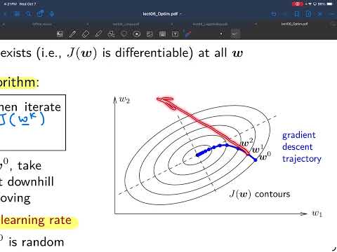
For an unconstrained differentiable objective J, gradient descent updates w^(k+1) = w^k − α_k∇J(w^k), starting from an initial w^0.
The positive step size α_k is also called the learning rate; each update moves downhill from the current parameter vector.
The gradient is perpendicular to objective contours, and repeated small steps can approach a nearby local minimum.
Because the update moves downhill, it generally cannot cross a higher-cost region to reach a deeper, distant minimum.

13:32 Why Random Initialization Avoids Getting Stuck at Stationary Points

Starting exactly at a maximum or saddle leaves gradient descent stuck because the gradient is zero and the update makes no change.
The lecture describes stationary points as a measure-zero set, so a random initialization almost surely does not land exactly on one.
Always initializing at zero can fail if a particular objective has a stationary point at zero; random starts reduce that risk.
Many machine-learning optimizers build on gradient descent and add speedups or other modifications.

17:00 Taylor-Series Argument for a Safe Gradient-Descent Step Size

A large step can overshoot a low-cost region and increase J, even when it initially points along the negative gradient.
Expanding J at w^k gives a change with a negative first-order term, −α_k‖∇J(w^k)‖², plus a higher-order term bounded by Cα_k²‖∇J(w^k)‖².
Balancing the terms at α_k = 1/C gives the boundary case; choosing a positive step size smaller than 1/C makes the first-order decrease dominate when the gradient is nonzero.
Since C is generally unknown, a fixed small learning rate is a simple practical choice; adaptive rates and changing the rate over time are also used.

30:00 Binary Logistic Regression as a Composition of Functions

The binary cross-entropy objective depends on sample scores z_i, each formed as the inner product of features and weights.
Adding a column of ones to the feature matrix gives A, so all scores can be computed together as z = Aw.
The objective is a sum of per-sample functions J_i(z_i), with each term depending on its training label y_i.
This separates the computation into a linear map from w to z and a nonlinear loss from z to J.

37:00 Multivariable Chain Rule as Gradient Flow Through a Computation Graph

For each weight w_j, the derivative sums contributions along all paths from w_j through the scores z_i to the scalar cost J.
Each score generally depends on many weights through a row of A, while each per-sample loss processes its own z_i before the losses are summed.
The same chain-rule procedure scales to layered neural networks and is automated by frameworks such as PyTorch and TensorFlow.

41:30 Logistic-Loss Derivatives Produce a Simple Matrix Gradient

Differentiating each binary cross-entropy term gives ∂J/∂z_i = σ(z_i) − y_i, where σ(z_i) = 1/(1 + e^(−z_i)).
Since z_i is the dot product of row i of A and w, its derivative with respect to w_j is A_ij.
Collecting the score derivatives into a vector yields ∇_w J = Aᵀ∇_z J = Aᵀ(σ(z) − y).
This matrix-vector form replaces an explicit sum over every training sample and feature.

45:29 Forward and Backward Passes for Logistic-Regression Code

The forward pass computes z = Aw, the sample probabilities σ(z), and the binary cross-entropy cost.
The cost can use the same probability-related quantities as the gradient, with algebraic rearrangement helping avoid repeated exponential calculations.
The backward pass forms the residual vector σ(z) − y and multiplies it by Aᵀ to obtain the weight gradient.
Tracking the cost at each gradient-descent iteration makes it possible to spot an excessive learning rate when the objective rises.

52:47 Cache the Feature Matrix with a Python Class

Rebuilding A inside the objective-and-gradient function wastes time and memory allocation when gradient descent calls it thousands of times.
A Python class can construct and store A once in __init__, alongside the training labels y.
A method such as J_eval then needs only the current weights w and can reuse self.A and self.y for each evaluation.
The next step is to call this cached objective-and-gradient method recursively within gradient descent.

Summary, takeaways, and chapters were generated by AI from the video's transcript and may contain errors. The video belongs to its creator, Prof. Schniter.