Lecture 12: Newton's method

Overview

Newton's method improves on steepest descent by minimizing a second-order Taylor approximation at each iteration, using the gradient and Hessian to choose an update. Burton Ma explains why this can converge in one step for a quadratic yet behave erratically when the Hessian is indefinite or ill-conditioned, then covers backtracking and the Levenberg-Marquardt modification, which shifts Hessian eigenvalues to make updates safer.

Key takeaways

Newton's update, w_(k+1) = w_k - H(w_k)^(-1)∇f(w_k), minimizes the local second-order Taylor model and can reach the exact minimum of a quadratic in one iteration.
A Newton direction is guaranteed to be a descent direction only when the Hessian is positive definite; an indefinite Hessian can point uphill even if backtracking reduces the step size.
Near-zero curvature can make Newton steps extremely large, while singular or ill-conditioned Hessians make the update undefined or numerically unreliable.
On the lecture's Rosenbrock example, undamped Newton converges in five iterations despite erratic steps and an objective increase; backtracking smooths the path but cannot repair an uphill direction caused by an indefinite Hessian.
Levenberg-Marquardt shifts Hessian eigenvalues by adding λI: small λ gives Newton-like behavior, while large λ produces a small steepest-descent-like step.
Dense Newton iterations require O(n²) Hessian storage and an O(n³) linear-system solve, so their rapid convergence must be weighed against computational cost in high dimensions.

Chapters

0:00 From Steepest Descent to a Second-Order Taylor Model

Steepest descent uses the negative gradient, but can zigzag around a minimizer; smaller steps reduce zigzagging at the cost of slower convergence.
A first-order Taylor approximation treats the function as locally linear, while Newton's method uses a second-order approximation that includes curvature.
The one-dimensional Taylor model is a parabola, whose minimum provides the next estimate of the function's minimizer.

5:30 Deriving the One-Dimensional Newton Update

Differentiating the Taylor parabola around the current point t_k and setting the derivative to zero gives t_(k+1) = t_k - f'(t_k)/f''(t_k).
The update is equivalent to derivative-based line search with direction -f'(t_k) and step size 1/f''(t_k).
Unlike a fixed-step gradient method, Newton's step size changes with the local second derivative.

11:00 When One-Dimensional Newton Steps Fail

If f''(t_k) is zero, the update is undefined; if it is near zero, the step can become enormous and cause divergence.
A negative second derivative makes the local Taylor parabola concave, so its stationary point is a maximum rather than a minimum.
Newton's method can converge unusually quickly in a bowl-shaped region, but a small change in the starting point can lead to divergence or oscillation.

15:00 Extending Newton's Method to Vectors and Hessians

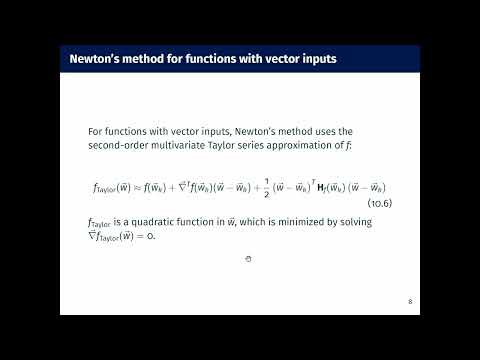
For a vector w, the second-order Taylor model uses the gradient transpose and the Hessian matrix H(w_k).
Setting the Taylor model's gradient to zero yields the multidimensional Newton update w_(k+1) = w_k - H(w_k)^(-1)∇f(w_k), when the Hessian is invertible.
The Newton direction is a descent direction when the Hessian is positive definite; positive definite matrices preserve the sign of the gradient's directional alignment.

22:00 Hessian Conditions and Solving Newton Systems

A negative definite Hessian points toward a local maximum, while an indefinite Hessian can produce either an ascent or descent direction.
A singular Hessian cannot be inverted, and an ill-conditioned Hessian can make the computed update numerically unreliable.
For implementation, solve H d = -∇f rather than explicitly computing H^(-1) and multiplying it by the gradient.

27:00 Quadratic, Gaussian, and Rosenbrock Newton Examples

For the convex quadratic f(w) = w1²/4 + w2², the second-order Taylor model is exact, so Newton's method reaches the minimum in one step from any starting point.
On the inverted Gaussian example, Newton's method reaches the minimum in about three iterations, with some oscillation.
On Rosenbrock's function, Newton's method takes large, erratic steps before entering the shallow valley, then converges in five iterations; one step increases the objective, unlike a guaranteed descent method.

31:40 Damped Newton Steps with Armijo Backtracking

Armijo backtracking can reduce the Newton step when the full update is too large, producing damped or relaxed Newton's method.
For the inverted Gaussian, damping reduces zigzagging and gives convergence in three iterations.
On Rosenbrock's function, backtracking produces a smoother path, but cannot fix a direction that is not a descent direction when the Hessian is indefinite.

36:00 Newton's Computational Cost and the Need for Hessian Fixes

In n dimensions, storing the Hessian requires O(n²) space, and computing its entries takes O(n²) operations.
Solving the Hessian linear system costs O(n³) with standard dense methods, making Newton's method expensive as n grows.
Indefinite or noninvertible Hessians motivate modifying the curvature matrix so that Newton-like updates remain usable.

40:40 Levenberg-Marquardt Shifts Hessian Eigenvalues

The Levenberg-Marquardt modification replaces H with H + λI, choosing λ large enough to make the modified matrix positive definite.
Adding λI shifts every Hessian eigenvalue by λ; as λ approaches zero, the update approaches Newton's method.
For large λ, the update approaches a small negative-gradient step, so intermediate values blend Newton's curvature information with steepest descent.
Levenberg proposed the approach in 1944; Marquardt reformulated and popularized it in 1963, especially for nonlinear least-squares optimization.

Summary, takeaways, and chapters were generated by AI from the video's transcript and may contain errors. The video belongs to its creator, Burton Ma.