ISE 754 (Fall 2026) 4.1 Shortest Paths and Road Networks

Overview

The lecture explains how to model road systems as weighted networks and use Dijkstra’s algorithm to find shortest paths, then applies network-processing operations to real logistics problems. It covers arc lists and adjacency matrices, graph structures, network thinning and facility connectors, and an interstate terminal-location model constrained by truck-driver hours of service.

Key takeaways

Road-network routing is more reliable than straight-line distance estimates when trips are under about 50 miles or when barriers such as mountains and major waterways affect available roads.
Arc lists can represent a legitimate zero-weight connection directly, while adjacency matrices may confuse zero weight with a missing arc; data and solver conventions must be checked.
Dijkstra’s algorithm is an efficient choice for road networks because road distances and travel times are nonnegative, but it is not appropriate for models that require negative arcs.
Thinning can make a national road network computationally manageable: the FAF example falls from roughly 35,000 nodes to 621 while preserving simplified interstate connections.
Route choice depends on the optimized weight: minimizing distance and minimizing travel time can produce different paths, as shown between High Point and Goldsboro.
Terminal placement must account for both local delivery reach and line-haul driver limits; the example adds an 11-hour hours-of-service constraint to a set-covering model and finds an 11-terminal solution.

Chapters

0:00 Road Networks: Nodes, Arcs, and Two Graph Representations

Great-circle distance with a circuity factor is a rough estimate that works best beyond about 50 miles and where waterways or mountains do not obstruct routes.
A road network represents intersections or facilities as nodes and road segments as arcs or links; arcs may be directed for one-way roads or undirected for two-way roads.
An arc list stores origin node, destination node, and weight vectors; weights commonly represent distance or travel time.
An adjacency matrix uses one row and column per node, with nonzero entries indicating arcs; a directed arc from node 3 to node 1 appears at position (3,1), not (1,3).

4:20 Bipartite Graphs, Zero-Weight Arcs, and Multigraphs

A complete bipartite graph links every node in one set to every node in another, such as manufacturing plants connected to distribution centers, with no links within either set.
Logistics networks may mix directed and undirected arcs; a zero-distance arc can represent a distribution center located at the same site as a plant.
Because zero in an adjacency matrix often means “no arc,” a genuine zero-weight arc may require special handling; some solvers, including Gurobi, interpret zero as absence.
A multigraph can retain multiple transport options between the same nodes, such as a low-cost pipeline with limited capacity and a more expensive truck alternative.

9:45 Dijkstra’s Algorithm and When Negative-Arc Methods Are Needed

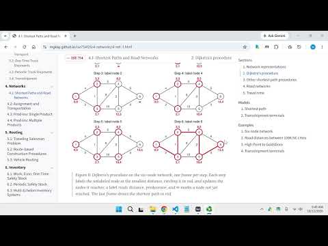
Dijkstra’s algorithm repeatedly labels the reachable unlabeled node with the smallest tentative distance, updating distances and predecessor nodes as shorter routes are found.
In the example from node 1 to node 6, node 2’s tentative distance improves from 4 to 3 via node 3; the final route has distance 13 and can be reconstructed by following predecessors backward.
Dijkstra’s method assumes all arc weights are nonnegative, which fits road distances and travel times.
Project scheduling can require negative arcs for maximum time-window constraints; Bellman–Ford or Floyd–Warshall can handle negative arcs, while Dijkstra is generally more efficient when its assumptions hold.

16:02 Thinning, Pruning, and Adding Facility Connectors

Thinning removes unnecessary degree-2 nodes and combines adjacent road segments; the Raleigh beltway example reduces alternative routes to the shorter clockwise path, yielding a 70-mile connection.
Thinning the FAF road network reduces roughly 35,000 nodes to 621 by removing non-interstate detail and simplifying road geometry.
Prune-and-reindex creates a subgraph for a selected area or arc filter—for example, retaining nodes inside a metro bounding box or arcs under 35 distance units—and renumbers the remaining nodes.
Add-connectors links facilities with known longitude and latitude to nearby road nodes using estimated distances; the default connector circuity factor is 1.3, compared with a typical 1.2 for broader estimates.

23:27 Travel-Time Routing and an Interstate Terminal-Location Model

The High Point–Goldsboro example distinguishes the shortest-distance route from the fastest route: changing network weights from distance to travel time can send traffic around Raleigh’s beltway.
For most logistics applications, minimizing travel time is the default objective, as in the first route typically offered by Google Maps.
A national LTL terminal-planning example uses the thinned interstate network and set covering to place transshipment terminals within 5.5 hours of interstate junctions.
An additional line-haul constraint requires travel between transshipment terminals to fit within the truck driver’s 11-hour driving limit; the mixed-integer model reports an optimal solution of 11 terminals.

Summary, takeaways, and chapters were generated by AI from the video's transcript and may contain errors. The video belongs to its creator, Michael G. Kay.