ISE 754 (Fall 2026) 3.3 Periodic Truck Shipments

Overview

Periodic shipment planning balances transportation charges against inventory carrying costs to find the shipment size that minimizes total logistics cost. Using a Raleigh-to-Gainesville example with annual demand of 20 tons, the analysis develops inventory-cost parameters and compares truckload and less-than-truckload options; the illustrated optimum is a 1.9-ton truckload shipment at about $28,000 annually, versus roughly $40,000 for the best LTL option.

Key takeaways

Periodic shipment planning must include inventory carrying cost: maximizing payload can lower transport cost while creating excess, obsolete, or spoiled inventory.
Keep fractional shipment frequencies in tactical planning; 3.27 truckloads per year is meaningful even though no single year will contain exactly 0.27 of a shipment.
Use the independent-shipment charge as a transport-cost upper bound and capacity-based full-truck allocation as a lower bound; actual consolidated rates generally lie between them.
Estimate inventory carrying rate h from interest, warehousing, and product-specific obsolescence; use α to represent the share of shipment value held in cycle stock.
Optimize truckload analytically and LTL numerically within the LTL regression’s valid range, then compare the separate optima to avoid a local-minimum error.
Aggregating the example’s 20- and 80-ton annual product demands cuts combined logistics cost from about $73,000 to just over $58,000.

Chapters

0:00 From One-Time Truck Quotes to Periodic Shipment Planning

A one-time operational decision chooses truckload or LTL for a known shipment; periodic planning instead chooses shipment size and frequency.
The Raleigh-to-Gainesville example adds annual demand of 20 tons to the prior lecture’s transportation data.
The calculated 3.27 truckloads per year is a planning average, not a count to round; rounding can distort results when the time unit changes.
Shipping at the 6.11-ton maximum payload gives an interval of about 111 days using 365.25 days per year.

7:00 Truckload Cost Bounds and the Three-Month Interval Constraint

Full-truckload frequency and the per-mile rate yield a monetary weight and an annual transport cost slightly above $4,000 for the example.
An interval constraint such as shipping at least every three months limits shipment size when full truckloads would arrive too infrequently.
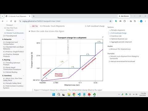
The independent-shipment curve is an upper bound on transport charges, while allocating a full truck’s cost by capacity share gives a lower bound.
Actual consolidated-carrier charges should fall between those bounds because carriers need profit and cannot always fill trailers exactly.

12:00 Modeling Inventory Carrying Cost with h and α

Total logistics cost combines transportation and inventory costs; purchase cost matters when comparing suppliers but can be omitted for a single supplier if shipment frequency does not affect it.
The inventory carrying rate h includes interest, warehousing, and obsolescence; 5% interest and 6% warehousing are suggested defaults absent better data.
The percent-reduction interval method estimates obsolescence from how quickly a product loses value, accommodating everything from perishable food to durable goods.
The inventory fraction α represents stock held across production, transit, and consumption: coordinated continuous production and consumption gives α = 1, while batch production followed by steady consumption gives α = 0.5.

20:00 Finding the Cost-Minimizing Truckload or LTL Shipment Size

Total logistics cost as a function of shipment quantity combines demand divided by quantity times the per-shipment transport charge with inventory carrying cost.
The truckload optimum has an EOQ-style analytical square-root solution; the LTL optimum requires numerical minimization because the rate regression has no closed-form solution.
LTL optimization must stay within the regression’s valid shipment-size range to avoid unrealistic extrapolation.
The example’s best truckload is 1.9 tons at about $28,000 in total logistics cost; the best LTL size is 0.76 tons at roughly $40,000.
Truckload and LTL should be optimized separately and their minima compared, since optimizing a combined, non-convex cost curve can stop at a local minimum.

27:00 Aggregating Periodic Shipments to Reduce Total Logistics Cost

Multiple products can be treated as one aggregate shipment using summed demand, demand-weighted value, and aggregate density and payload inputs.
For the two-product example, optimizing shipments separately costs about $73,000, while aggregation reduces total logistics cost to slightly over $58,000.
The aggregate’s density, value, and maximum payload fall between the individual products’ values, as expected from the weighted calculations.
Aggregation changes shipment sizes and frequencies: it slightly increases the first product’s shipment size while substantially reducing the second product’s.

Summary, takeaways, and chapters were generated by AI from the video's transcript and may contain errors. The video belongs to its creator, Michael G. Kay.