fnb100f261020

Overview

Jeff Hunk introduces Module 3 on the time value of money, building from annual compounding to present value and discounting, then deriving the geometric average or CAGR formula by isolating the rate with fractional exponents. He applies the ideas in Excel, comparing annual and quarterly compounding and showing how to solve for future value, present value, and APR while keeping periodic rates and compounding periods distinct.

Key takeaways

The compound-growth model FV = P × (1 + r)^n supports both forward projections and reverse valuation: discounting gives P = FV ÷ (1 + r)^n.
At 10% annual growth, $1,000 becomes about $2,594 in 10 years, while 5% annual inflation makes a future $1,000 worth about $614 today.
The annualized growth rate is derived as r = (FV/PV)^(1/n) − 1 by isolating the exponent with an nth root and then subtracting 1.
For quarterly compounding, divide APR by 4 to obtain the periodic rate and multiply years by 4 to obtain the number of periods.
When solving for a quarterly rate but reporting APR, multiply the periodic rate by the compounding frequency; the two rates are not interchangeable.
At the same principal, APR, and time horizon, quarterly compounding produces a greater future value than annual compounding because interest is applied four times per year.

Chapters

0:00 Class Begins: Module 3 and the Time Value of Money

Jeff Hunk opens the Tuesday class by introducing Module 3, the time value of money.
He connects the new topic to geometric averages introduced in Topic 1.
The lesson reviews compounding before moving into valuation and Excel exercises.

4:00 Snowball Growth and the Compound Interest Formula

Jeff uses a snowball gathering more snow as it rolls downhill to illustrate compounding.
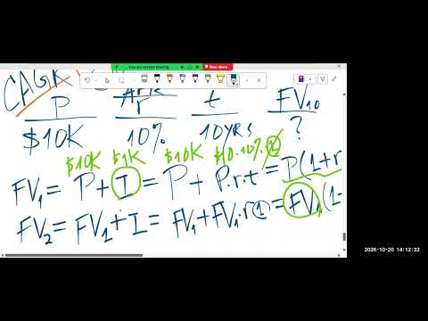
For a $10,000 principal at a 10% annual rate, year-one value is $11,000.
Applying the same growth factor again gives the year-two value, establishing the pattern of multiplying by 1 + r each year.

7:30 Deriving Future Value as Principal Times One Plus Rate to n

Repeated annual growth leads to the general formula FV = P × (1 + r)^n.
Here, P is the starting principal, r is the annual interest rate, and n is the number of years.
Jeff distinguishes capital-market compounding from the simple-interest convention he associates with short-term money markets.

13:00 Why $1,000 Today Is Worth More Than $1,000 in Ten Years

At a 10% annual return, $1,000 today grows to about $2,594 after 10 years.
With 5% annual inflation, $1,000 received in 10 years has a present purchasing-power value of about $614.
The comparison illustrates how investment returns and inflation both compound over time.

19:10 Time Value of Money as Finance’s Valuation Foundation

Jeff’s course introduction describes financial-asset valuation as the present value of future cash flows discounted at a required rate of return.
The discount rate reflects the tradeoff between consumption today and the expected benefits of saving or investing.
The module covers cash-flow patterns, unknown rates and time periods, exponents, logarithms, and Excel-based actuarial calculations.

22:00 Present Value and Discounting Reverse Compounding

Compounding solves for future value when principal, rate, and time are known; discounting solves for principal when future value is known.
Rearranging FV = P × (1 + r)^n gives P = FV ÷ (1 + r)^n.
Jeff identifies compounding and discounting as reverse processes and links discounting to the earlier inflation example.

29:00 Inflation, Investment Returns, and the Four Unknowns

Jeff explains that an investment earning 10% annually grows faster than prices rising at 5% annually.
The base formula has four variables that can be unknown: future value, principal or present value, rate, and number of periods.
He poses examples including growing $100,000 to $1 million and estimating how long that goal takes at a 25% or 30% return.

37:00 CAGR Recalled as the Solution for the Unknown Rate

Jeff recalls the geometric-average formula from Topic 1: r = (FV ÷ PV)^(1/n) − 1.
The formula is also described as compound annual growth rate, or CAGR.
He begins deriving it from FV = P × (1 + r)^n rather than treating it as a formula to memorize.

43:00 Fractional Exponents Turn Roots into Algebra

Jeff reviews how square roots, cube roots, and fourth roots undo powers of 2, 3, and 4.
He writes an nth root as a fractional exponent, such as x^(1/n).
He also reviews that negative exponents represent reciprocals, for example x^(-2) = 1/x².

53:00 Deriving the CAGR Formula by Isolating the Rate

Starting from FV/PV = (1 + r)^n, raise both sides to the power 1/n to remove the exponent n.
Subtracting 1 yields r = (FV/PV)^(1/n) − 1.
Jeff emphasizes applying the same operation to both sides of an equation and using logical algebra instead of memorizing the result.

57:00 Opening the Module 3 Single Cash Flow Excel Worksheet

Jeff directs students to download the Module 3 Excel file and select the tab labeled “Single Cash Flow.”
He checks that students have opened the worksheet before beginning the calculations.
The spreadsheet examples cover future value, present value, and rate calculations.

1:02:00 Quarterly Compounding: Adjust APR and Count Periods

The worksheet compares a $10,000 deposit earning 10% APR for 10 years under annual and quarterly compounding.
For quarterly compounding, the periodic rate is APR divided by 4, or 2.5%, and the period count is 10 × 4 = 40.
The quarterly calculation produces a higher future value because interest is applied more frequently.

1:06:40 Excel’s Consistent Formula Structure for Compounding

Jeff keeps the annual case in the same spreadsheet structure by using a compounding frequency of 1.
For quarterly calculations, he separates periodic rate and total periods, then uses FV = P × (1 + r)^N.
Consistent formulas can be filled down across repeated examples, while restoring erased cell borders keeps the worksheet presentable.

1:11:00 Checking Present Value Formulas Against the Starting Deposit

The worksheet discounts a target future value over 10 years at 10% to recover the starting principal.
For quarterly compounding, the formula uses the periodic rate and 40 total periods.
Jeff checks that discounting returns the original $10,000, confirming the calculation reverses the earlier compounding example.

1:13:30 Solving for APR with Annual and Quarterly Compounding

For a $10,000 investment that triples in five years, the annual-compounding rate is found with the CAGR formula.
With quarterly compounding, first solve for the quarterly periodic rate using 20 periods, then multiply by 4 to report APR.
Jeff warns that the unconverted quarterly rate is not the annual percentage rate required by the worksheet label.

1:19:00 Compounding Frequency Changes the APR Needed for a Target

For the same principal, time horizon, and target future value, more frequent compounding allows a lower APR.
Jeff explains this as the interest rate working more frequently, consistent with the higher future value from quarterly compounding at the same APR.
He closes by checking students’ Excel results and confirming participation.

Summary, takeaways, and chapters were generated by AI from the video's transcript and may contain errors. The video belongs to its creator, Jeff Hunk.