fnb100f261019a

Overview

Jeff Hunk introduces time value of money by connecting compounding, discounting, inflation, and present value, then guides students through Excel examples for annual and quarterly compounding. He also derives the CAGR formula by solving the future-value equation for the rate, while encouraging students to learn investing with small amounts rather than treating his own NASDAQ-heavy portfolio's roughly 15% historical annualized return as a guarantee.

Key takeaways

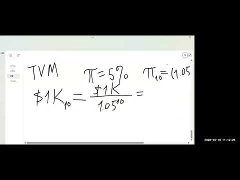
At 5% annual inflation, $1,000 received ten years later has a present value of about $614, calculated as $1,000 ÷ 1.05^10.
Compounding uses future value = principal × (1 + periodic rate)^total periods; discounting rearranges the same equation to find present value.
For a 10% APR compounded quarterly, the periodic rate is 2.5%, and a 10-year term contains 40 compounding periods.
A $1 million goal in 10 years at a steady 15% annual return requires about $247,000 invested initially, assuming the return compounds at that rate.
CAGR is derived by solving the compound-growth equation for the rate: (future value ÷ present value)^(1/n) − 1.
Jeff Hunk recommends beginning to learn about investing with small amounts, such as $100, and treats his portfolio's roughly 15% annualized five-year performance as a personal example rather than a guaranteed outcome.

Chapters

0:00 Class Begins with Attendance and Quiz One Reminders

Jeff Hunk welcomes students, checks attendance, and asks participants to turn on their cameras.
He reminds the class to submit Quiz One before introducing the next module.

3:20 Module Three Connects Time Value of Money to Compounding

Jeff Hunk opens Module Three, Time Value of Money, after completing Module Two.
He links the new topic to compounding and geometric averages introduced in Topic One.

5:17 Why $1,000 Today Is Worth More Than $1,000 in Ten Years

Jeff Hunk contrasts receiving $1,000 now with receiving the same nominal amount ten years later.
At 5% annual inflation, he discounts the future $1,000 by 1.05 raised to the tenth power.
The future payment is worth about $614 in today's dollars, illustrating present value.

10:10 Compounding Turns Principal and Interest into Future Value

Jeff Hunk distinguishes compounding, which calculates future value, from discounting, which brings future value back to present value.
He illustrates compounding with a $10,000 principal earning 10%: the balance reaches $11,000 after year one and $12,100 after year two.
The general formula is future value = principal × (1 + rate)^number of periods.
His snowball analogy describes how earned interest itself earns additional interest as the balance grows.

19:45 Solve for Present Value to Reach a $1 Million Goal

Rearranging the future-value formula gives present value = future value ÷ (1 + rate)^time.
For a $1 million target in 10 years at a 15% annual return, the required starting amount is about $247,000.
Jeff Hunk describes his own portfolio as having doubled over five years, equivalent to roughly 15% annualized, and says it is heavily weighted toward NASDAQ-related investments.
He notes that his portfolio contains about 60 individual stocks and ETFs, and that its growth made it too substantial to treat as a low-stakes experiment.

26:30 Learn Investing with a Small Brokerage Account

Jeff Hunk recommends beginning with a small amount, such as $100, rather than taking large risks.
He names Robinhood, E-Trade, and Charles Schwab as brokerage examples and suggests considering an S&P 500 ETF.
He argues that investing firsthand can help students observe how interest rates, inflation, AI news, and market volatility affect prices.
His bicycle analogy emphasizes learning through manageable mistakes instead of starting with an expensive investment.

32:40 Open the Single Cash Flow Excel Worksheet

Jeff Hunk directs students to download the Module Three Excel exercise and open the first worksheet, labeled Single Cash Flow.
He asks students to confirm the file is open using a green check mark and takes a class screenshot.
The worksheet is used to calculate future and present values under different interest and compounding assumptions.

40:00 Calculate Annual Compounding for a $10,000 Deposit

The first Excel example starts with $10,000, a 10% APR, and a 10-year timeline.
With annual compounding, the future-value calculation is $10,000 × (1 + 0.10)^10, or about $25,937.
Jeff Hunk defines compounding frequency as the number of times interest is added each year, such as 1 annually, 2 semiannually, 4 quarterly, or 12 monthly.
He distinguishes relatively steady account interest from daily stock-price changes, whose returns fluctuate.

44:30 Quarterly Compounding Adjusts Both Rate and Period Count

For a 10% APR compounded quarterly, the periodic rate is 10% ÷ 4, or 2.5% per quarter.
A 10-year investment compounded four times per year has 40 total compounding periods.
Jeff Hunk explains that more frequent compounding produces a higher future value when the APR and investment term remain the same.
He distinguishes the number of years from the total number of compounding periods.

48:10 Simplify Excel Formulas with Periodic Rate and Period Columns

Jeff Hunk adds spreadsheet columns for periodic rate and total compounding periods to make formulas easier to inspect.
The quarterly example uses APR divided by 4 and 10 years multiplied by 4, then applies principal × (1 + periodic rate)^periods.
He recommends consistent spreadsheet structure so formulas can be checked and reused more easily.
Dragging a formula down fills calculations for multiple scenarios, and he restores the outside border to keep the worksheet professionally formatted.

52:00 Use the Same Excel Structure to Discount Future Cash Flows

The class reverses the future-value calculation to find the principal needed today for a specified future amount.
For quarterly discounting, the rate is adjusted by dividing APR by the quarterly frequency, and the exponent reflects the total periods.
Jeff Hunk keeps the same worksheet structure for annual and quarterly cases, even when a frequency of 1 does not change the result.
He asks students to verify that their spreadsheet results match before taking another screenshot.

58:18 Ten-Minute Class Break

Jeff Hunk pauses the lesson for a ten-minute break after the Excel exercise.
He asks students to remain connected and keep their cameras on, with a profile picture as an alternative.

1:12:30 Review Compounding and Discounting as Inverse Processes

After the break, Jeff Hunk restates future value as principal multiplied by (1 + rate) raised to the number of periods.
Solving for principal yields present value, so compounding and discounting reverse one another.
He frames rate and number of periods as additional possible unknowns in the same equation.

1:16:40 Set Up the Unknown-Rate and Unknown-Time Questions

For an unknown rate, the example asks what return would grow $100,000 to $1 million in 10 years.
For an unknown time period, the example holds the $100,000 principal, $1 million target, and an assumed 25% annual return constant.
Jeff Hunk identifies four quantities that can be solved for: future value, present value, rate, and number of periods.

1:20:00 Connect Topic One's Geometric Average to CAGR

Jeff Hunk recalls that Topic One introduced annualized return, geometric average, and CAGR as related concepts.
CAGR means compounded annual growth rate and is calculated as (future value ÷ present value)^(1 ÷ number of years) − 1.
He now derives the formula from the compounding equation instead of treating it as a formula to memorize.

1:23:20 Use Fractional Exponents to Undo the Compounding Power

To isolate the rate in future value = present value × (1 + rate)^n, Jeff Hunk first divides by present value.
He explains that raising both sides to the power of 1/n removes the exponent n.
The explanation reviews how fractional exponents represent roots, such as a square root as a one-half power.
His numerical check compares (2^2)^3 with 2^(2×3), with both expressions equaling 64.

1:30:40 Derive the CAGR Formula by Isolating the Rate

Raising both sides of future value ÷ present value = (1 + rate)^n to the power of 1/n leaves 1 + rate on the right.
Subtracting 1 gives rate = (future value ÷ present value)^(1/n) − 1.
Jeff Hunk identifies this result as CAGR or geometric average for the single-growth scenario discussed.

1:33:00 Review Assigned Videos and Close the Class

Jeff Hunk asks students to watch all assigned videos and notes that the material has been condensed into a two-hour session.
He says the next class will continue with the exercise and reminds students of the October 27 deadline.
The class ends with a reminder to meet again on Wednesday.

Summary, takeaways, and chapters were generated by AI from the video's transcript and may contain errors. The video belongs to its creator, Jeff Hunk.