EAS4200 Aerospace Structures, Lecture 23, 2026 fall

Overview

Ting Dong develops a fatigue-crack-growth workflow using the Paris law: relate crack-growth rate to stress-intensity range, integrate from an observed crack size to the critical size, and estimate remaining cycles to fracture. The lecture explains threshold and fracture limits, Mode I toughness, compressive-load treatment, and the geometry-factor iteration, then applies the method to a plate example.

Key takeaways

The Paris law, da/dN = C(ΔK)^m, estimates stable fatigue-crack growth using material constants and the stress-intensity range.
Remaining life begins at the inspected crack size ai; it does not include cycles before crack detection or initiation.
For a compressive minimum stress, use zero as the effective minimum when calculating Paris-law stress range, but use σmax to determine the critical fracture size.
The fracture limit follows K₁c = βσmax√(πaf), linking material toughness and maximum load to the crack size at failure.
Because β depends on af through the plate geometry ratios, the critical-size calculation is iterative; the classroom shortcut starts with β = 1 and recalculates once, while real engineering analysis iterates to convergence.

Chapters

0:00 Fatigue Crack Growth, Stress Intensity, and the Three Growth Regimes

Crack-growth rate is expressed as da/dN, where a is crack size and N is the number of load cycles.
The stress-intensity range ΔK depends on stress range, crack size, and a geometry factor; growth is negligible below the threshold ΔKth.
The crack-growth curve has three regimes: near-threshold growth, stable propagation, and unstable propagation leading to fracture.
Mode I opening is identified as the main crack mode considered in the course, with failure when its stress intensity reaches K₁c.

4:45 Paris Law for Stable Crack Propagation

In the stable middle regime, experimental data are approximated by a straight line on a log-log plot.
The Paris equation is da/dN = C(ΔK)^m, where C and m are material constants.
Substituting ΔK = βΔσ√(πa) connects crack growth to stress range, crack size, and geometry factor β.
The lecture uses the Paris-law region because the near-threshold and unstable regimes are not suitable for the same stable-growth calculation.

8:30 Integrating Paris Law from the Measured Crack to Failure

Separating crack-size terms from cycle terms allows integration from initial crack size ai to final crack size af.
The resulting cycle count estimates remaining life from the time a crack is detected, not from the original crack-initiation event.
Required inputs include the measured crack size, material constants C and m, stress range Δσ, and geometry factor β.
The final crack size is determined separately using the fracture criterion based on K₁c.

13:30 Compressive Stress and the Effective Fatigue Stress Range

When minimum stress is compressive, the lecture treats the compressive portion as non-promoting for crack growth and sets the effective minimum to zero.
For Paris-law calculations in that case, use Δσ = σmax rather than subtracting the negative minimum stress.
Ting Dong connects this convention to the Goodman mean-stress treatment: compressive mean stress does not reduce the equivalent alternating stress.
The stress range governs ΔK and crack growth, while σmax is used separately for the critical final-crack calculation.

19:00 Finding Critical Crack Size with Mode I Toughness K₁c

The final crack size af is found by setting βσmax√(πaf) equal to the material’s Mode I fracture toughness K₁c.
Using maximum stress gives a conservative fracture limit across the loading cycle.
K₁c acts as the fracture threshold, analogous to a strength limit in a static-load failure calculation.
The initial crack size is the crack measured during inspection; af is the calculated size at which fracture is expected.

22:15 Resolving the Geometry-Factor Dependency by Iteration

The geometry factor β depends on crack-size ratio a/B and plate ratio H/B, but af itself must be calculated using β.
A full numerical solution repeats the process: assume β, calculate af, read a new β from the geometry chart, and continue until af converges.
For coursework, use the simplified procedure: start with β = 1, calculate af, read β again from the chart, then recalculate af once.
For engineering work, continue iterations until successive values are nearly unchanged rather than stopping after the classroom approximation.

31:20 Plate Example: Set Geometry, Material, and Loading Inputs

The worked example uses a square plate with 10-inch dimensions, 0.5-inch thickness, and an initial through-thickness crack of 0.075 inch.
The problem supplies tensile and compressive loading, Paris-law constants, and K₁c, then asks for remaining cycles before fracture.
Maximum tensile stress is calculated as tensile force divided by the plate cross-sectional area, using 0.5 × 10 inches.
The example begins the final-size calculation with β = 1, then uses af/B and H/B to select a revised β from the chart.

37:00 Complete the Example with Revised β and Paris-Law Integration

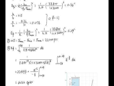
The example reads a revised geometry factor of approximately 1.1 from the chart and recalculates the critical crack size.
Because the minimum load is compressive, the stress range is taken as maximum stress minus zero for the Paris-law integration.
The remaining-life calculation integrates from the given 0.075-inch initial crack to the calculated final crack size, using the supplied C, m, and stress range.
The lecture ends by evaluating the integral for the plate example and inviting questions about the procedure.

Summary, takeaways, and chapters were generated by AI from the video's transcript and may contain errors. The video belongs to its creator, Ting Dong.