CS3130FS26Module3R1VidProc

Overview

The lecture reviews algorithm-analysis problems and emphasizes proving answers with constructions and careful operation counts rather than intuition. Key methods include sharing intermediate powers and applying Horner’s rule to evaluate polynomials, using the optimal comparison bound ⌈3n/2⌉ − 2 to find a minimum and maximum, and simplifying constrained problems before restoring their conditions.

Key takeaways

A higher polynomial degree does not guarantee a higher multiplication count: repeated squaring evaluates x^16 in 4 multiplications, so degree alone cannot establish a universal cost claim.
For the polynomial with exponents 7, 16, 25, 34, and 43, factoring x^7 and substituting y = x^9 enables a 10-multiplication evaluation when powers are shared and Horner’s rule is used.
Finding both the minimum and maximum of 99 elements requires at least ⌈3·99/2⌉ − 2 = 147 comparisons under the optimal bound.
When a problem supplies known relationships, solve the unrestricted version first and then restore the conditions; subtract a saved comparison only if its information fully replaces a comparison the original method needs.
For a(x) + b(x), combine coefficients of like powers before applying Horner’s rule; separately evaluating both polynomials can waste multiplications.
In the 12-element constrained inversion example, the 10 unrestricted elements contribute 45 inversions, while reinserting x4 and x10 adds 6 and 4, producing 55 total.

Chapters

0:00 Universal Claims and the Polynomial-Degree Counterexample

A statement labeled true must hold in every case; one counterexample is enough to make a universal claim false.
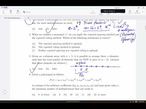
The claim that higher-degree polynomials always require more multiplications is false: evaluating x^16 by repeated squaring takes 4 multiplications.
Treat broad claims as useful problem-solving principles, but check for exceptions rather than assuming they are mathematical laws.

2:00 Repeated Squaring and Why Degree Does Not Determine Cost

Repeatedly squaring x computes x^2, x^4, x^8, and x^16 in 4 multiplications.
A polynomial such as 1 + x^16 shows that the example still applies when the expression has multiple terms.
Operation counts depend on the available computation strategy, not just on the polynomial’s degree.

6:09 Constructing a Permutation with Exactly Three Fixed Elements

To demonstrate a permutation with n − 3 elements out of place, first fix three elements in their original positions.
Circularly rotate the remaining elements by one position so each moves away from its original position.
Constructing examples—and counterexamples—is a practical way to test claims instead of relying on a guess.

11:50 Shared Powers and Horner’s Rule for a Ten-Multiplication Polynomial

Factor out x^7 from terms with exponents 7, 16, 25, 34, and 43; the remaining exponents are multiples of 9.
Set y = x^9, turning the remaining expression into a degree-4 polynomial that Horner’s rule evaluates in 4 multiplications.
Prepare x^7 and x^9 together by reusing x^2 and other intermediate powers; the preparation takes 5 multiplications.
Count one additional multiplication outside the Horner evaluation: 5 preparation + 4 Horner + 1 final product = 10.

20:34 Comparing Large Expressions with Exponent Laws

Rewrite 100 as 10^2 and apply (a^m)^n = a^(mn) before taking a base-10 logarithm.
Use known bounds such as 2^10 = 1,024 > 1,000 to compare very large powers without evaluating every digit.
Wolfram|Alpha was recommended as a symbolic-calculation aid and described as permitted for the test, while algebraic reasoning remains important.

27:13 Simplifying Nested Logarithms with a Substitution

For expressions involving repeated logarithms, substitute x = log n to expose their simpler structure.
The compared forms become x^2 and x ln x; comparing them is easier than tracking the original nested logarithms.
The same substitution strategy can help compare more complicated expressions, including logarithms that appear in fractions.

31:05 Optimal Comparisons for Finding Both a Minimum and a Maximum

The optimal comparison count for finding both the minimum and maximum among n elements is ⌈3n/2⌉ − 2.
For n = 99, the bound is ⌈148.5⌉ − 2 = 147 comparisons; no method can do it in 146.
When evaluating a proposed comparison budget, a value at least as large as the bound is sufficient under the stated result; a smaller value is impossible.

37:02 Midterm Structure and Preparing for Nontrivial Variations

Part A covers the first 10 questions in formats such as multiple choice, true/false, and short answers; Part B covers 10 basic computation questions.
The in-class assessment was scheduled for the following Wednesday, with homework questions serving as starting points for modified problems.
Expect nontrivial changes to conditions, not merely replacement numbers; understanding the original solution is needed to adapt it.
Online tools may support studying, but obtaining an answer without understanding the reasoning will not prepare students to solve independently.

43:14 The Golden Rule: Simplify First, Then Restore Given Conditions

Temporarily ignore a given condition to solve a simpler version, then bring the condition back and account for its effect.
For the n = 11 minimum-and-maximum example, the unrestricted bound is ⌈3·11/2⌉ − 2 = 15 comparisons.
Three supplied inequalities can save three comparisons only when they fully replace comparisons that the tournament method would otherwise need.
Some conditions provide only partially useful information, so subtracting every stated comparison can produce an incorrect estimate.

49:27 Mixing Repeated Squaring and Cubing to Share Powers

For monomial evaluation, consider both repeated squaring and repeated cubing; an exponent’s structure determines which is more useful.
When a polynomial has two terms such as a·x^49 + b·x^54, compute x^49 and reuse it to obtain x^54 by multiplying by x^5.
Plan intermediate powers so required results such as x^5 are shared rather than computed independently.

53:17 Pascal’s Triangle, Binomial Expansion, and Combined Horner Evaluation

Identify the Pascal’s triangle coefficients to rewrite the target as a binomial expression such as (a(x) + b(x))^5.
Do not evaluate a(x) and b(x) separately if their like powers can be combined first.
Combine corresponding coefficients—for example, combine the x² coefficients as a₂ + b₂—then apply Horner’s rule to the resulting polynomial.
Combining terms avoids redundant multiplications by sharing computation before evaluation.

56:54 Constrained Inversions: Simplify the Array Before Counting

For a maximum-inversion problem, descending order gives the unrestricted maximum; the lecture warns that this is only the first step when elements have placement constraints.
For the 12-element example, remove the constrained x4 and x10 temporarily, leaving 10 elements whose descending arrangement has 10·9/2 = 45 inversions.
Restore the conditions afterward and count the additional inversions contributed by each reinserted element.

58:40 Reinserting x4 and x10 Adds Ten Inversions

Inserting x4 adds 3 inversions with larger elements before it and 3 with smaller elements after it, for 6 total.
Inserting x10 adds 2 inversions on each side, for 4 total.
The constrained arrangement therefore has 45 + 6 + 4 = 55 inversions; count the effects of each restored element explicitly.

Summary, takeaways, and chapters were generated by AI from the video's transcript and may contain errors. The video belongs to its creator, DrHeUMSLTeaching.